Sage Journals: Discover world-class research

Abstract

In dense wireless sensor networks, density control is an important technique for prolonging the network's lifetime while providing sufficient sensing coverage. In this paper, we develop three new density control protocols by considering the tradeoff between energy usage and coverage. The first one, Non-Overlapping Density Control, aims at maximizing coverage while avoiding the overlap of sensing areas of active sensors. For the ideal case, a set of optimality conditions are derived to select sensors such that the sensing space is covered systematically to maximize the usage of each sensor and minimize the coverage gap. Based on theoretical optimality conditions, we develop a distributed protocol that can be efficiently implemented in large sensor networks. Next, we present a protocol called Non-Overlapping Density Control Based on Distances that does not require location information of the nodes. This protocol is more flexible and easier to implement than existing location-based methods. Finally, we present a new range-adjustable protocol called Non-Overlapping Density Control for Adjustable Sensing Ranges. It allows heterogenous sensing ranges for different sensors to save energy consumption. Extensive simulation shows promising results of the new protocols.

Keywords

Sensor Networks Topology and Density Control Distributed Algorithms Network Reconfiguration

1. Introduction

Many sensor network applications require sensors to monitor and collect data in a region of interests. These applications usually require a certain coverage, if not complete coverage, to ensure that the area is taken care of. Due to limited energy resources in each sensor node, sensors are usually deployed in high density and take turns to work in order to prolong the network lifetime [1]. Density control techniques have been developed to determine when and which sensors should be powered up and which should be put into an energy saving mode, so that energy is saved while the active nodes form a connected network and cover the sensing space well.

One approach to prolonging the network lifetime and saving energy is to divide the operating time into many rounds and set different nodes active in different rounds depending on their energy levels and other attributes [19]. In the beginning of each round, all the nodes in the network make their decisions to turn ON or OFF. When the nodes with higher energy levels are given higher priority to turn on, the energy consumption across the nodes will be balanced out. A core of this approach is the method for determining the “on” nodes in each round.

Different applications require different degrees of sensing coverage. While some applications may require a complete coverage in a region, others may only need a high percentage coverage. For example, distributed object tracking and detection may require that every location be monitored [5]. Environment temperature and humidity monitoring may only need approximate information around a certain location. This approximation does not require every location to be covered. Among existing density control protocols, some are designed for complete coverage [19], [15] whereas others are not [18], [9]. In reality, complete sensing coverage is difficult due to the irregular sensing areas of sensors, the topology of the network, and the dynamic conditions of the environment. Thus, although it is a common practice in protocol design to model the sensing area as an ideal disk, the result will be an approximation of the real situation.

In this paper, we consider the tradeoff between energy usage and coverage and develop new distributed density control protocols to improve performance. The rest of this paper is organized as follows. In Section 2, we review the existing work on density control. In Section 3, we analyze the optimal conditions for the new density control strategy in the ideal case and present three new protocols. In Section 4, we show the experimental results of the new protocols. Finally, in Section 5, we conclude the paper.

2. Related Work

Many topology and density control methods have been proposed for wireless sensor networks [2], [3], [4], [14], [17], [18], [19]. In [17], GAF divides the region of interest into virtual grids, and one node in each grid is selected to be “on” in each round. CEC follows the same principle of GAF by selecting working nodes in a cluster-based model. They are the first experiment on topology control over real hardware. In Ascent [2], each node self-determines its participation based on its contribution to network connectivity by checking its local node density and measuring message loss rate. In PEAS (Probing Environment and Adaptive Sleeping) [18], sleeping nodes wake up once in a while to probe their neighborhood and replace any failed working node. The method is ad hoc, and the decision time for each node in every round is usually very long.

For mobile sensor scenarios, methods have been proposed to move mobile sensors so that coverage gaps can be filled [14]. The mobile sensors can even adjust their sensing coverage on the fly. The costs of mobile sensors and moving them during operation are usually very high, requiring expensive hardware and software support. Sensor placement methods have also been proposed to optimize the number of sensors and locations [3]. A theoretical analysis of the problem of estimating redundant sensing areas among neighboring sensors shows that partial redundancy is more realistic for real applications as complete redundancy is expensive [4].

Mathematical programming and computational geometry techniques have been applied to density control. In [6], a centralized ILP (Integer Linear Programming) method is presented to find a minimal set of active nodes that can completely cover a sensing space, which is solved as 0/1 scheduling problems. In [7], a centralized method is proposed to use a Voronoi diagram and Delaunay triangulation to find a minimal exposure path (i.e., a path connecting two points which maximizes the distance of the path to all sensor nodes) and a maximal exposure path (i.e., a path connecting two points which maximizes the smallest observability of all the points on the path) in a network graph, respectively.

Recently, the relationship between coverage and connectivity has been studied, and it is proved that if the radio range is at least twice that of the sensing range, a complete coverage of a convex area implies connectivity among the working set of nodes [15], [19], [13]. Thus, when the condition is satisfied, the topology control problem is simplified and becomes a sensing coverage problem. In [19], an optimal geographical density control protocol, called OGDC, is proposed based on the optimality conditions under which a subset of working sensor nodes can be chosen for complete coverage.

It is proved that the problem of finding a maximal number of covers in a sensor network is NP-complete [12]. Several approximate methods are developed. In practice, adaptive and heterogeneous sensing range adjustment is preferred. However, optimal density control for heterogeneous sensing ranges is much harder than homogeneous sensing range cases. Although OGDC is extended to include different sensing ranges in [19], the calculation is complicated and no distributed algorithm is presented. In addition, the extended OGDC does not deal with adjustable sensing ranges. In [16], two density control methods for adjustable sensing ranges are proposed, but they are centralized algorithms.

In this paper, we analyze the trade-offs between sensing area overlap and sensing gaps and present three protocols with unique features that improve existing density control protocols.

3. Three New Density Control Protocols

Monitoring a larger physical space using sensor networks generally means more working (active) sensor nodes and more energy usage. Our design strategy for optimal density control is to maximize the return of energy spending or the average coverage per working node while relaxing the requirement of covering the whole space.

3.1 Non-Overlapping Density Control Protocol (NODC)

The primary goal of NODC is to minimize the uncovered area (sensing gaps of the working nodes), while avoiding overlaps of the sensing areas of working nodes. The benefit is that, compared to OGDC, NODC generates solutions of much fewer working nodes with only a slight degradation of the sensing coverage, a higher average coverage per working node, and leading to prolonging the lifetime of the network significantly.

In the ideal case, we derive the optimal conditions for NODC based on the following assumptions:

The sensing area of each node is represented as a disk of the same size. Although this “cookie-cutter” approach is overly simplistic for real applications, it is useful in understanding and analyzing the basic properties of protocols and thus has been used in most of the previous work.

Sensor node density is sufficiently high that a sensor can be found at any desirable point.

The interested sensing space is much larger than the sensing range of each sensor node so that the boundary effects can be ignored.

The radio range is at least twice the sensing range. This assumption works for the types of sensors with a small localized sensing range, such as passive sound sensors detecting signals stronger than a certain threshold.

Each node knows its position. Most existing protocols are designed based on knowing node locations. In the latter part of the paper, we will present a new protocol that does not require this information.

Although the analysis is for homogenous sensing ranges, it can be easily extended to heterogenous sensing range cases.

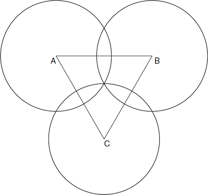
A representative case of three working nodes selected according to the criteria of NODC is shown in Fig. 1, where the sensing areas of the three nodes (represented as disks) just touch each other and the sensing gap (the uncovered area) between the working nodes is minimized. The sensing gap inside the equilateral triangle ΔABC is $(\sqrt{3} - \frac{π}{2}) r_{s}^{2}$ , where r_s is the sensing range, the radius of the disk. The ratio of the uncovered area to the area of the triangle ΔABC is $1 - \frac{π}{2 \sqrt{3}} = 9.31 %$ , which equals the ratio of the uncovered space to the whole sensing space if the sensing space is very large compared to the sensing range of each node and all nodes are placed according to the pattern in Fig. 1.

Figure 1

The main idea of NODC: Minimizing the sensing gap between adjacent working nodes (nodes A, B, and C) while avoiding overlap of their sensing areas. Circles A, B and C are just tangent with each other.

In contrast, the goal of the existing protocol OGDC [19] is to minimize the overlaps of the sensing areas of working nodes (cannot make it zero), while avoiding sensing gaps. Figure 2 shows the example of the ideal case of OGDC for three working nodes. The overlapping area in the equilateral triangle ΔABC is $(\frac{π}{2} - \frac{3 \sqrt{3}}{4}) r_{s}^{2}$ . The ratio of the overlapping area to the area of the triangle is $\frac{2 π}{3 \sqrt{3}} - 1 = 20.9 %$ , which equals to the ratio of the overlapping space to the whole sensing space if the sensing space is very large compared to the sensing range of each node and all nodes are placed according to the pattern in Fig. 2. The amount of overlap is quite significant in this case.

Figure 2

The main idea of OGDC: Minimizing the overlap of sensing areas of adjacent working nodes (nodes A, B, and C) while achieving complete coverage. The cross point of circles A and B is just covered by circle C.

In the rest of this section, we present the detailed implementation of the distributed protocol. The overall process of NODC is similar to OGDC. At any time, a node is in one of the three states: “UNDECIDED,” “ON,” and “OFF” time is divided into rounds. At the beginning of each round, all nodes wake up, set their states to “UNDECIDED,” and carry out the process of selecting the working nodes. The process ends when all the nodes change their states to either “ON” or “OFF.” All nodes remain in the state until the beginning of the next round. NODC applies a new strategy in selecting working nodes in each round.

3.1.1 Selection of the Starting Nodes

At the beginning of each round, every node is powered on in the “UNDECIDED” state. A node volunteers to be a starting node with a certain probability if its power exceeds a pre-determined value P_t, which is related to the length of the round and in general is set to a value so as to ensure with high probability that the sensor can remain powered on until the end of the round.

If a sensor node volunteers, it sets a backoff timer of τ₁ seconds, where τ₁ is uniformly distributed in some range. When the timer expires, the node changes its state to “ON” and broadcasts a power-on message. If a node hears other power-on messages before its timer expires, it cancels its timer and does not become a starting node. The power-on message sent by the starting node contains

(i)
the position of the sender and
(ii)
the direction a along which the second working node should be located.

This direction is randomly generated from a uniform distribution in [0, 2π].

If a node does not volunteer itself to be a starting node, it sets a timer of T_s seconds. T_s should be set to a sufficiently large value such that the operation of selecting working nodes can complete if there is at least one starting node.
3.1.2 Actions Taken When a Node Receives a Power-On Message

When a sensor node receives a power-on message, if its power is less than P_t, it turns itself off and sets its state to “OFF;” otherwise, it checks whether or not the ratio of its sensing area covered by its “ON” neighbors to its overall sensing area is over a predetermined threshold (the turn-off threshold). If so, it sets its state to “OFF” and turns itself off. Otherwise, it adds this sender to its active neighbor list and takes actions according to the following rules R1 to R4.

Rule R1: The message is the first power-on message received and is from a starting node. A node tells whether or not a message was sent from a starting node by the value set in the direction field α: if α ≥ 0, then the message was originated from a starting node. In this case, the node sets a timer of T_c1 seconds. When the timer expires, the node sets its state to “ON” and broadcasts a power-on message (with α set to a negative value). If the node hears any other power-on message before its timer expires, it carries out the operations specified in Rule R3.

Figure 3

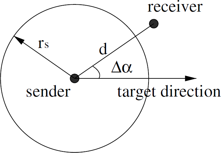
An illustration of the parameters of formula T_c1 in Eq. (1).

The value, T_c1, of the backoff timer is set as follows:

T_{c 1} = t_{0} (c ((2 r_{s} - d)^{2} + (d Δ α)^{2}) + u),

(1)

where t₀ is the time it takes to send a power-on message, c is a constant that determines the backoff scale, d is the distance from the sender to the receiver, Δα is the angle between α and the direction from the sender to the receiver, as shown in Fig. 3, and u is a random number drawn from the uniform distribution [0,1].

Rule R2: The message is the first power-on message received but is from a non-starting node. If the value carried in the direction field, α, of the power-on message is negative, then the message was originated from a non-starting node. In this case, the node sets a timer of T_e seconds, where the value of T_e is much larger than that of T_c1.

Rule R3: The message is the second power-on message received. If the coverage areas of the two senders do not intersect, then if the second sender is farther away from the receiver than the first one, the receiver simply ignores the new message but retains the timer set for the first power-on message; otherwise, it cancels the existing T_e or T_c1 timer and sets a timer of T_c1 based on the second sender. If the two senders intersect, the receiver cancels the existing timer and sets a timer of T_c2 seconds.

Figure 4 illustrates the basic idea for computing T_c2. Let O denote the crossing point of the coverage areas of the two senders, C the optimal location of a third sensor node to just touch the area covered by nodes A and B, R the location of the receiver node, d the distance between the node and the crossing point O, and Δα the angle between $\bar{O C}$ and $\bar{O R}$ . Then the value of T_c2 is

T_{c 2} = t_{0} (c ((\bar{O C} - d)^{2} + (d Δ α)^{2}) + u),

(2)

where

\bar{O C} = \sqrt{(2 r_{s})^{2} - {(\frac{1}{2} \bar{A B})}^{2}} - \frac{1}{2} \bar{O O^{1}}

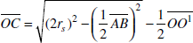
and t₀, c, and u are the same as in Eq. (1). When the timer expires, the node sets its state to “ON” and broadcasts a power-on message with α set to a negative value. If the node receives any other power-on message before its timer expires, it carries out the operations specified in Rule R4.

Figure 4

An illustration of the parameters of formula T_c2 in Eq. (2).

Rule R4: More than two power-on messages have been received. This case can be further divided into three subcases.

None of the coverage areas of the senders overlaps with each other. The receiver keeps the current timer unchanged.

The coverage areas of the previous senders do not overlap, but the coverage area of the new sender overlaps with at least one of the coverage areas of the previous senders. Find the previous sender that is closest to the receiver and overlaps with the new sender. Set the timer of the receiver to a new T_c2 value computed based on this previous sender and the new sender.

The coverage areas of the previous senders overlap and the coverage area of the new sender also overlaps with at least one of the coverage areas of the previous senders. If the new sender is closer to the receiver than the previous senders, find the previous sender that is closest to the receiver and overlaps with the new sender and set the timer of the receiver to a new T_c2 value computed based on this previous sender and the new sender. Otherwise, keep the current timer unchanged.

Figure 5 shows the results of NODC and OGDC on a randomly generated deployment. Two hundred sensor nodes are randomly deployed inside a 50m by 50m square region. The region is divided into 50 × 50 grids. A grid is considered covered if the center of the grid is covered. The sensing range of each node is 5m. The time it takes to send a power-on message t₀ is 7ms. The constant c used in Eqs. (1) and (2) is $10 / r_{s}^{2}$ . The other parameters are set to the same values for OGDC as in [19]. The turn-off threshold θ is 1. For each node, if the fraction of its sensing area covered by other nodes is equal to or larger than θ, the node turns itself off.

Figure 5

Example of NODC and OGDC. Δ represents sensor nodes; · (dot) represents the center of a grid; × represents a grid that is covered; and the circle represents the sensing area of the starting node, node 18. The dark × (or red in the original color image) represents the covered area by the current node.

In the figure, Δ represents sensor nodes; · (dot) represents the center of a grid; × represents a grid that is covered; and the circle represents the sensing area of the starting node, node 18. The dark × (or red in the original color image) represents the covered area by the current node.

The coverage of NODC and OGDC is shown after 10 nodes are turned on. The results show that NODC expands its coverage faster, but is more likely to leave some small sensing gaps.

The computation and communication complexity of the protocol is very low. The computation is asynchronous, and each node makes its own decision based on its condition and available information heard over the radio. The most expensive computation by each node is computing the backoff timer values, which consists of simple arithmetical operations. The communication cost consists of broadcasting the node locations and power-on messages. Each node only needs to broadcast its own location once and a power-on message once. The protocol has a convergence rate of O(log n), where n is the number of nodes, and generally converges quickly in practice.

3.2 Non-Overlapping Density Control Protocol Based on Distances (NODCD)

Most existing density control protocols require each node to know its locations, at least its relative location to its neighbors. In some applications, the location information may be hard or expensive to get, or the locations estimated using localization algorithms may not be accurate [8], [11], [10]. In this section, we present a new protocol called Non-Overlapping Density Control Based on Distances, NODCD, that does not require the location information. It performs density control purely based on the distances to the local neighbors of each node. The protocol is very simple, yet achieves good results.

NODCD can be viewed as a simpler version of the NODC protocol presented in the last section. It uses the following two rules to determine the backoff timer of each node.

Rule R1′: The message is the first power-on message received. The receiver sets its timer to a value of T′_c1 in Eq. (3).

T_{c 1}^{'} = t_{0} (c (2 r_{s} - d)^{2} + u),

(3)

where the parameters t₀, c, d, and u have the same meaning as in Eq. (1). If the node hears any other power-on messages before its timer expires, it carries out the operations specified in Rule R2′.

Rule R2′: More than one power-on messages have been received. If the new sender is the closest to the receiver among the previous senders, then the receiver sets its timer to a value of T′_c1 in Eq. (3) computed based on the distance to the new sender. Otherwise, the receiver keeps its timer unchanged.

Note that in both rules, the only information required is the distance between the receiver and the sender.

Figure 6 shows the result of NODCD in the same example as in Fig. 5 after 10 sensor nodes are turned on. The example shows that NODCD expands its coverage faster than NODC and leaves more sensing gaps.

Figure 6

An example of NODCD. Δ represents sensor nodes, · (dot) the center of a grid, and × a grid that is covered.

3.3 Density Control with Adjustable Sensing Ranges (NODCA)

Most existing density control protocols assume the sensing ranges of all the sensors are identical. In [16], two node scheduling models are proposed to utilize the adjustability of sensing ranges in order to minimize the energy consumption. However, their algorithms are centralized. Using a similar idea, we develop a new protocol called Non-Overlapping Density Control for Adjustable sensing ranges (NODCA).

In NODCA, each node decides whether it turns itself off based on a threshold, θ ∊ [0,1]. For each node, if the fraction of its sensing area covered by other nodes is equal to or larger than θ, the node turns itself off. Then, given a target θ, 0 ≤ θ ≤ 1, and a maximum sensing range r_s, NODCA goes through several iterations, and in each iteration NODCD is called with an increasing turn-off threshold and a decreasing sensing range. For example, the NODCD protocol with two iterations is as follows:

Run NODCD with turn-off threshold θ₁, θ₁ < θ, and sensing range r_s. All nodes use the same turn-off threshold and sensing range. Because the turn-off threshold is smaller than the target, some nodes are turned off earlier.

Reset the states of the “OFF” nodes after the first step to “UNDECIDED” and run NODCD again with turn-off threshold θ and sensing range r₂, r₂ < r_s. A smaller sensing range leads to less energy consumption. The idea is that if the sensing gaps of the working nodes turned on in Step 1 are small, then we should use smaller sensing disks (the sensing area of each node) to fill the gaps. Larger sensing disks will create a lot of overlaps with existing working nodes and waste energy.

One question is how to determine θ₁ and r₂. In our experiments, we set θ₁ = θ − 0.1 and $r_{2} = \frac{1}{\sqrt{3}} r_{s}$ . The r₂ value is set according to the analysis of the two adjustable sensing range models in [16]. The optimal values of θ₁ and r₂ are left for future work. The 2-step NODCA is used in our experiments.

In terms of energy consumption, we only consider the energy used in sensing, not including the power consumed by radio communication and computation. We apply two energy models in our evaluation, in which the power consumption is proportional to $r_{s}^{2}$ and $r_{s}^{4}$ , respectively. For n working sensors with sensing ranges r_(s,i), 1 ≤ i ≤ n, and the sensing area A, the models describe the total sensing energy consumption of the sensors per area. They are

Energy Model I

E_{1} = \frac{\sum_{i = 1}^{n} r_{(s, i)}^{2} μ_{1}}{A}

(4)

Energy Model II

E_{2} = \frac{\sum_{i = 1}^{n} r_{(s, i)}^{1} μ_{2}}{A}

(5)

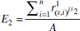
where μ₁ and μ₂ are power consumption parameters. When we present the energy usage in the experimental results, if E₁ = μ₁, we call it one energy unit of model I. Similarly, if E₂ = μ₂, we call it one energy unit of model II. The actual values of μ₁ and μ₂ are not important when we compare the relative performance of the different protocols.

Fig. 7 shows the result of the two-iteration NODCA on the same example as in Fig. 5 after the first iteration, i.e., running NODCD with turn-off threshold 0.9 (Note that the final turn-off threshold is 1). The figure shows that the majority of the space has been covered. The remaining small gaps will be handled in the second iteration, using a smaller sensing range (smaller energy usage by the working node) with turn-off threshold 1 (corresponding to complete coverage).

Figure 7

An example of the two-iteration NODCA after the first iteration. Δ represents sensor nodes, · (dot) the center of a grid, and × a grid that is covered. The dark × (or red in the original color image) represents the covered area by the current node, the first node being turned on in the second iteration.

4. Experimental Results

In the simulations, we compare the three new protocols with OGDC. The parameters of the networks are set mostly to the same values as in the OGDC experiments in [19]. Since their differences are in the working node selection process at the beginning of each round, we only compare their selection results of one round. We assume all the power-on nodes with the same sensing range will cost a certain same amount of energy and all the sleeping nodes will not cost any energy. We also assume each node's lifetime is much longer than the round time in which a subset of nodes working together, and it is much longer than the time all the nodes finish making their decisions from the “UNDECIDED” state to the “ON” or the “OFF” state. Thus, the overhead of density control is relatively small enough.

Specifically, the parameters are as follows:

The region of interest is a 50m by 50m square.

The sensing range of each node r_s is 5m. It is the maximum sensing range in the adjustable sensing range experiments.

The time it takes to send a power-on message t₀ is 7ms.

The constant c used in Eqs. (1) and (2) is $10 / r_{s}^{2}$ .

The other parameters are set to the same values for OGDC as in [19].

The coverage is measured as follows: the area is divided into 50 × 50 grids. A grid is considered covered if the center of the grid is covered. The coverage is defined as the ratio of the number of grids that are covered by at least one sensor to the total number of grids.

In the experiments, 100 random instances are used for each case, and the average results are reported. In each run, the nodes are randomly deployed in a uniform way in the region of interest. All protocols start with one starting node. The protocols are implemented in MATLAB.

4.1 NODC and NODCA

According to previous research, coverage and energy are two of the most critical issues in wireless sensor networks. Thus the performance metrics we use are

(i)
the percentage of coverage, i.e., the ratio of the covered area to the total area of interest;
(ii)
the number of working nodes required to provide the percentage of coverage in (i); and
(iii)
the sensing energy based on energy model I, Eq. (4), and model II, Eq. (5).

When the sensors are homogeneous, the number of working nodes in the network is directly proportional to the energy consumption of the network.

In the simulation, we compare the results of three protocols, NODC, NODCA, and OGDC, for different power-off thresholds of the nodes. For each node, when the fraction of its sensing area covered by other nodes is above the power-off threshold, it turns itself off.

Figures 8 and 9 show the results of the four performance metrics versus the turn-off threshold percentage for sensor networks with 150 and 300 sensor nodes. Between NODC and OGDC, OGDC gives better coverage, but uses more working nodes. When the turn-off threshold is set to 100%, each node only turns off when its sensing area is completely covered. For this case, both protocols achieve about the same coverage. They use similar number of working nodes when the network is a less dense (the 150-node cases), and OGDC uses fewer working nodes when the network is dense (the 300-node cases).

Figure 8
Performance comparison of NODC, NODCA, and OGDC on sensor networks with 150 nodes.

Figure 9
Performance comparison of NODC, NODCA, and OGDC on sensor networks with 300 nodes.

As the turn-off threshold decreases, the overall coverage decreases, but at a much slower rate than the turn-off threshold. For example, when the turn-off threshold is 50% in the 150-node cases, i.e., a node turns itself off if half of its sensing area is covered, the overall coverages of NODC and OGDC are 85% and 88%, respectively, much larger than 50%. On the other hand, the numbers of working nodes needed are 34 and 41, respectively, just about half of the numbers (around 75) needed for achieving full coverage. More working nodes are needed when the turn-off threshold increases.

When the turn-off threshold is less than 100%, NODC uses fewer working nodes than OGDC, and the difference increases as the turn-off threshold decreases. The saving of working nodes by NODC against OGDC goes up to 25%. At the same time, the reduction of the overall coverage of NODC against OGDC is less than 5%. In many applications, it is worthwhile to trade the small reduction of coverage with the significant saving of working nodes. The relative performance of NODC and OGDC is generally the same for networks of different densities.

The adjustable sensing range protocol, NODCA, indeed saves more energy. The benefit comes from the smaller sensing range used by NODCA in the second step. Among the three protocols, NODCA uses the least amount of energy for all the different network densities and turn-off thresholds. Compared to OGDC, NODCA consistently saves over 20% energy according to both energy models. The coverage is almost the same as OGDC when the turn-off threshold is high, especially for dense networks. Compared to NODC, NODCA consistently saves a significant amount of energy according to energy model II. When the turn-off threshold is low, they use about the same amount of energy according to energy model I. The energy saving is large for both energy models when the turn-off threshold is high. NODCA achieves slightly better coverage than NODC for dense networks (the 300-node case) and is about the same for the 150-node networks.

The completion time of the working node selection process of the three protocols is comparable and all small. Compared to the relatively long round time, the overhead of density control is small in all three protocols.
4.2 NODCD

We now present the results of NODCD, using OGDC as a reference. Note that NODCD only uses distance information between neighbors, while OGDC uses node locations. Because NODCD uses less information than OGDC, it is not really a fair comparison of their performance if only distance information is available.

The performance metrics we use are the percentage of coverage and the number of working nodes required to provide the coverage. In the experiments, the sensors are homogeneous, so the number of working nodes in the network is directly proportional to the energy consumption.

We show the results of NODCD and OGDC for different power-off thresholds of the nodes. The power-off condition is defined differently from the previous section. Because NODCD only uses distance information, the power-off condition for each node is also defined based on distance, not the fraction of its sensing area covered by other nodes. Actually, without knowing node locations, the fraction of coverage cannot be calculated.

The power-off condition is defined as follows. Given a power-off threshold β and the sensing range r_s, for each node, if $\frac{3}{2} - \frac{d}{r_{s}} \geq β$ , where d is the distance of the node to its closest working node, then the node turns itself off.

In our experiment, β takes on values in [0, 1]. When β = 0, a node turns itself off if there is a working node within $\frac{3}{2} r_{s}$ distance. When β = 1, a node turns itself off if there is a working node within $\frac{1}{2} r_{s}$ distance.

Figure 10 shows the results for sensor networks with 150, 200, and 300 sensor nodes. By only using distance information, NODCD can achieve very good results. Compared to OGDC, NODCD uses slightly fewer working nodes and has slightly less coverage. When the turn-off threshold is high, e.g., 100%, NODCD has almost the same result as OGDC, in terms of both coverage and number of working nodes. When the network is less dense (the 150-node case), their difference is also very small when the turn-off threshold is low. Another benefit of NODCD is its simplicity and ease of implementation.

Figure 10

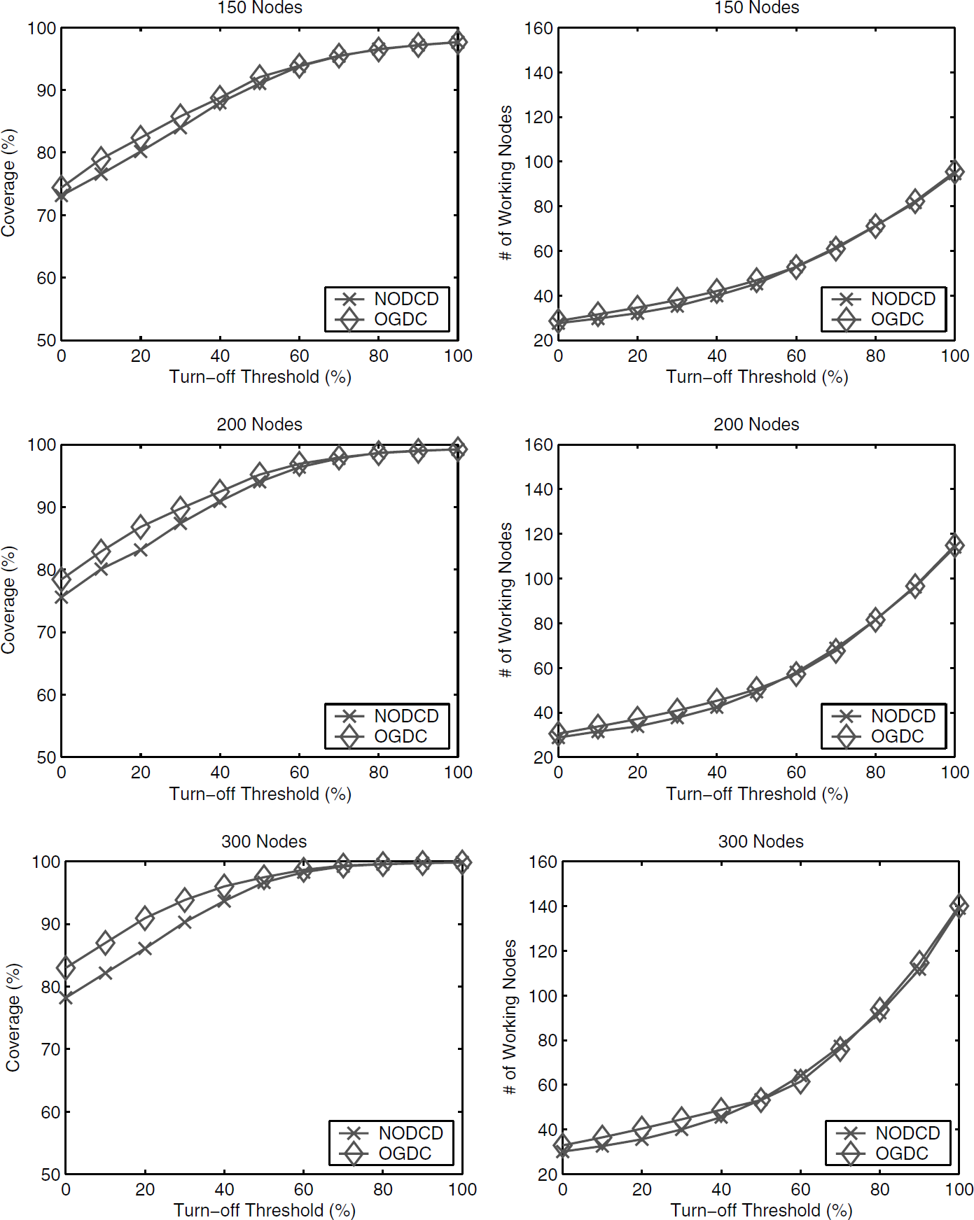
Performance comparison of NODCD and OGDC on sensor networks with 150, 200, or 300 nodes.

5. Conclusions

In this paper, we have presented three new density control protocols that apply new strategies in trading the coverage vs. energy usage, without using node locations, and saving energy by taking advantage of adaptive sensing ranges. The protocols are distributed, easy to implement, and have low computation and communication costs. We compare their performance with the existing protocol, OGDC, showing significant improvement in the number of working nodes and energy consumption. The new protocols are attractive in applications where complete coverage is not necessary, difficult to achieve, or each node has a different, possibly irregular, sensing range. We plan to further analyze the protocols and derive better parameters.

Most of the density control approaches are based on geometric location information. However, protocols solely based on deployment knowledge do not require additional energy cost to obtain location information [4]. One future direction is to combine node localization techniques and density control techniques so that effective density control can be carried out on networks even without distance information.

Footnotes

Acknowledgement

The work presented in this paper was partially supported by the National Science Foundation under grant CNS-0423386.

References

Akyildiz

I. F.

Sankarasubramaniam

, and Cyirci

. “Wireless sensor networks: A survey.” In Computer Networks, vol. 38(4), 393–422, March 2002.

Cerpa

and Estrin

. “Ascent: Adaptive self-configuring sensor networks topologies.” In Proc. IEEE INFOCOM'2002, New York, NY, USA, June 2002.

Dhillon

S. S.

and Chakrabarty

. “Sensor placement for effective coverage and surveillance in distributed sensor networks.” In Proc. IEEE Wireless Communications and Networking Conference, 1609–1614, 2003.

Gao

, and Li

. “Analysis on the redundancy of wireless sensor networks.” In Proceedings of the 2nd ACM international conference on Wireless sensor networks and applications, 108–114. ACM Press, 2003.

Wong

Y. H.

, and Sayeed

. Detection, classification and tracking of targets in distributed sensor networks. In IEEE Signal Processing Magazine, Volume: 19 Issue: 2, March 2002.

Megerian

and Potkonjak

. Low power 0/1 coverage and scheduling techniques in sensor networks. In UCLA Technical Reports 030001, January 2003.

Meguerdichian

Koushanfar

Potkonjak

, and Srivastava

M. B.

. Coverage problems in wireless ad-hoc sensor networks. In Proc. IEEE INFOCOM', April 2001.

Niculescu

and Nath

. Ad-hoc positioning system. In IEEE GlobeCom, Nov. 2001.

Shakkottai

Srikant

, and Shroff

. Unreliable sensor grids: Coverage, connectivity and diameter. In Proc. IEEE INFOCOM', San Francisco, USA, 2003.

10.

Shang

and Ruml

. “Improved MDS-based localization.” In Proc. IEEE InfoCom, March 2004.

11.

Shang

Ruml

Zhang

, and Fromherz

. “Localization from mere connectivity.” In ACM MobiHoc, 201–212, Annapolis, MD, June 2003.

12.

Slijepcevic

and Potkonjak

. “Power efficient organization of wireless sensor networks.” In IEEE International Conference on Communications, vol. 2, 472–476, 2001.

13.

Tian

and Georganas

N. D.

. “Connectivity maintenance and coverage preservation in wireless sensor networks.” In Proc. of the 2004 IEEE Canadian Conference on Electrical and Computer Engineering, 2004.

14.

Wang

Cao

, and La Porta

. “A bidding protocol for deploying mobile sensors.” In Proceedings of the 11th IEEE International Conference on Network Protocols, 315. IEEE Computer Society, 2003.

15.

Wang

Xing

Zhang

Pless

, and Gill

. “Integrated coverage and connectivity configuration in wireless sensor networks.” In First ACM Conference on Embedded Networked Sensor Systems (SenSys'03), Los Angeles, CA, November 2003.

16.

and Yang

. “Coverage and connectivity in sensor networks with adjustable ranges.” In International Workshop on Mobile and Wireless Networking (MWN), 2004.

17.

Bien

Mori

Heidemann

, and Estrin

. “Topology control protocols to conserve energy inwireless ad hoc networks.” Technical Report 6, University of California, Los Angeles, Center for Embedded Networked Computing, January 2003. submitted for publication.

18.

Zhong

, and Zhang

. “Peas: A robust energy conserving protocol for long-lived sensor networks.” In Proceedings of the 10th IEEE International Conference on Network Protocols, 200–201. IEEE Computer Society, 2002.

19.

Zhang

and Hou

. “Maintaining coverage and connectivity in large sensor networks.” In International Workshop on Theoretical and Algorithmic Aspects of Sensor, Ad hoc Wireless and Peer-to-Peer Networks, Feb 2004.

Flexible Energy Efficient Density Control on Wireless Sensor Networks

Abstract

Keywords

1. Introduction

2. Related Work

3. Three New Density Control Protocols

3.1 Non-Overlapping Density Control Protocol (NODC)

4.1 NODC and NODCA

Footnotes

Acknowledgement

References