Sage Journals: Discover world-class research

Abstract

Sensor network research is still in its infancy. There is a large volume of exploratory research. From lack of experimental data and sophisticated models derived from such data, many sensor network publications continue to use data generated from simple models in their algorithm evaluation. It is commonly agreed that data processing algorithms in sensor networks are sensitive to input data. However, no previous efforts have been devoted to quantitatively characterize the range of the algorithm performance when evaluated using different data input.

In this paper, we made the first attempt to quantify the algorithm's sensitivity to data. Our evaluation results demonstrated that different data input could change the algorithm performance by as much as an order of magnitude or even change the relative performance order of two alternative algorithms. This pointed out the need to evaluate sensor network systems with data representing a wide range of real-world scenarios. For each algorithm in our case study, we identified a small set of data characteristics essential to the algorithm's performance. This defined a unique feature of our synthetic data generation framework and made both synthetic data generation and evaluation scalable. To support systematic algorithm evaluation and robust algorithm design and deployment, our synthetic data generation toolbox can generate 1. irregular topology data based on empirical models which will maintain important features of the experimental data; and 2. data corresponding to a wide range of parameter values.

Keywords

Scalable Synthetic Data Generation Systematic Algorithm Evaluation Robust Algorithm Design Search Space Reduction Data Sensitivity Sensor Networks

1. Introduction

It is commonly agreed that data processing algorithms in sensor networks are sensitive to input data. However, no previous efforts have been devoted to quantitatively characterize the range of the algorithm performance when evaluated using different data input. Due to lack of experimental data and sophisticated data models, many sensor network publications continue to use data generated from simple models in their algorithm evaluation. For example, it is common that data collection and estimation algorithms are evaluated with uniform or Gaussian data input [11, 31]. Similarly, a random Gaussian field model is typically used in both analytical and simulation studies to evaluate the compression and source coding algorithms [16].

If various data input generated from different models (ranging from simple models to complex or empirical models) only produce small perturbations on the algorithm performance, simple models are preferred. This is justified by the Akaike Information Criteria (AIC) [18]. Unfortunately, the type of input data and node topology used in the evaluation often significantly influence the evaluation results.

In this paper, we quantified the extent of this data sensitivity problem through statistical performance analysis and evaluation. Using case studies of two concrete sensor network algorithms, we demonstrated that different data input could change the algorithm performance by an order of magnitude, or even change the relative performance order of two alternative algorithms.

We would like to clarify that the objective of our case studies was not meant to criticize any particular algorithms. Rather our objective was to demonstrate potential problems in the evaluation methodology followed by many sensor network researchers, i.e., evaluating algorithms only based on data generated from simple models. As a result, we recommend evaluating sensor network algorithms with data representing real-world scenarios or data corresponding to a wide range of conditions. Generating data satisfying the above requirements presented several challenges:

Scalability Issues The parameter space is huge in fully characterizing a physical phenomenon. The following back-of-the-envelop calculation demonstrated that the search space in the synthetic data generation is at least exponential. A spatial data set with m possible sensor readings each at n locations has mⁿ possibilities in the synthetic data output. Further, sensor data input is often 8 or 16 bits, in which case, m = 2⁸ or m = 2¹⁶. Thus, systematic algorithm evaluation by exhaustive search is not practical.

Reality Check Ideally, algorithm evaluation using our synthetic data will provide insight on system performance in future field deployments; therefore, the synthetic data is desirable to represent real world scenarios. We wanted to avoid the pathological scenarios in which the synthetic data misguides the simulation.

Unavailability of Ideal Experimental Data Most existing experimental data are collected from a regular grid; however, sensor networks are usually deployed in an ad-hoc manner. Evaluating algorithms with irregular topology data versus regular grid data could lead to completely different results [40]. Therefore, existing experimental data cannot be directly used to evaluate sensor network algorithms.

To address the above challenges, we proposed two strategies: First, through concrete case studies, we identified a small number of parameters essential to algorithm performance. This will significantly reduce the search space in synthetic data generation. Second, we used empirical models derived from experimental data to guide simulation towards those portions of the space that represent real world scenarios. Guided by these two strategies, we adopted two complementary techniques to generate synthetic data of an arbitrary irregular topology: trace based and analytical model based approach. In the trace based approach, we used empirical models to guide synthetic data generation towards those portions of the parameter space that represented real world scenarios. The synthetic data generated from this approach will have similar characteristics as the experimental data trace. When the available experimental data is scarce, we used analytical models with adjustable parameters to generate synthetic traces exhibiting a wide range of data characteristics over the parameter of interest to applications. The second approach also allowed us to investigate how a single parameter affects the algorithm performance while the other parameters remain fixed.

From the conceptual point of view, our main contributions fall into the following categories:

Systematic evaluation methodology to quantify the algorithm's sensitivity to data and deduce a small number of essential parameters to a given algorithm. This is illustrated through two case studies.

When the algorithm performance can be attributed to a single parameter, we used non-parametric statistical tools and experimental data to examine how the algorithm performance varies with the changing parameter value.

When the algorithm performance depends on multiple parameters, we used synthetically generated scenarios to investigate changes in performance with each parameter. In the synthetically generated scenarios, we have the flexibility to vary the phenomena along a single dimension while keeping other parameters fixed.

Search space reduction in synthetic data generation. Systematic algorithm evaluation also helped to identify a small set of data characteristics essential to algorithm performance. Identifying a small set of essential data features allowed us to focus on the important features in the synthetic data generation, thus reducing the search space significantly from exponential to a manageable number.

In general a fair understanding of the algorithm under evaluation and some preliminary algorithm evaluations helped to identify the relevant set of data features. The systematic performance evaluation techniques introduced in Sections 2 and 3 are used to verify whether there is a strong correlation between the identified data feature and the algorithm performance.

Organization of the Paper

We start the paper with two case studies: 1. percentile estimation of the field data, and field estimation. 2. In percentile estimation, the algorithm performance can be attributed to a single parameter (see evaluation results in Section 2).

For field estimation, there has been extensive research in sampling and reconstruction of a physical field [32, 37, 5, 26] in recent sensor network literature. We investigated Fidelity Driven Sampling in Section 3. Fidelity Driven Sampling represented a fairly complex algorithm, its performance depended on multiple parameters. These case studies served two-fold purposes: First, these algorithms served as examples of systematically studying the dependency of algorithm performance on data. Second, for each case study, we identified a small set of parameters essential to the algorithm performance. Identifying a small number of essential parameters helped to achieve scalability in both synthetic data generation and evaluation.

Section 4 contains the implications of these case studies to a scalable synthetic data generation framework and our synthetic data generation techniques. We review related work in Section 6. Section 7 discusses the general applicability of our proposed evaluation methodology and how it can be applied in evaluating a new algorithm.

2. Statistics Estimation Applications

We considered a type of algorithm in which we are able to identify a single parameter that determines the algorithm performance. In particular we presented results on percentile estimation algorithms. We studied two types of percentile computation algorithms [21, 28], and identified a single parameter, p-percentile bin size, essential to the algorithm performance. In the case of percentile estimation by uniform sampling, we proved that p-percentile bin size is sufficient to determine the algorithm performance. This sufficiency proof significantly reduced the search space in synthetic data generation.

2.1 Sensitivity of Algorithm Performance on Data and Identification of Essential Data Characteristics

2.1.1 Median Computation by Uniform Sampling

For simplicity of illustration, we considered an instantiation of random process Z(u) as deterministic. Given a snapshot of sensor readings at each node (z(i), i = 1,…, n), in an ascending or descending order, the real median M(Z) is defined as $z (\frac{n + 1}{2})$ if n is odd; or $(z (\frac{n}{2}) + z (\frac{n}{2} + 1)) / 2$ if n is even. The estimated median is written as M(Z).

Random Sampling provides a simple aggregation technique for in-network processing. There are variations of median estimation by uniform sampling. Without loss of generality, we considered a specific median computation by a uniform sampling algorithm as follows:

a single sink in the deployed sensor network and each sensor node has the same probability (e.g., 1%) of sending its reading back to the sink.

the sensor value is forwarded along the shortest path tree from the sensor source to the sink. Further, an intermediate node on the shortest path tree simply relays these packets back to the sink.

p samples are transmitted back to the sink, s(1),…, s(p); The real median M(Z) is estimated by the median M(S) of s(1),…, s(p).

By using statistical tools we systematically investigated the algorithms performance across a wide range of data distributions. Our statistical analysis consisted of three key steps.

First, we defined our performance metric to be normalized estimation error—the difference between the estimated median, µ(Z), and the real median, M(Z), normalized by the range of the entire set of sample values. Normalization is introduced to make comparing results across different data sets meaningful. Often, the median is used as a robust estimator instead of mean. Therefore, we defined the error metric in terms of value, as opposed to position.¹

Second, we identified the relevant data characteristic to be normalized median bin size. We bin the entire set of samples into a fixed number (e.g., 10) of equally spaced containers. Median bin is defined as the container that includes the median. Let n denote the total number of samples, and m denote the number of samples in the median bin, then the normalized median bin size is defined as m/n.

Last, we quantified the range of algorithm performance with data input of various parameter values. We evaluated the algorithm using two types of data: data simulated from Gaussian, Exponential, and Weibull distributions; and 259 snapshots of S-Pol radar data.² The S-Pol radar data recorded the intensity of reflectivity in dBZ, where Z is proportional to the returned power for a particular radar and a particular range. We selected 259 time snapshots across 2 days in May 2002 in our study. Each snapshot is a 60 × 60 spatial grid data with 1 km spacing.

Note that data generated from simple models have been widely used in sensor network publications. We varied the parameters in the above models across a wide range: Gaussian distribution—fixed mean and varied standard deviation from 1 to 100; Weibull distribution—fixed scale parameter and varied shape parameter from 1 to 100; Exponential distribution—varied exponential changing rate λ from 0.1 to 10.

Figure 1 shows the scatter plot of the normalized estimated median error vs. the normalized median bin size. Each point in the graph corresponded to results averaged from 100 runs of the algorithm on a single data set. The x-axis is the normalized median bin size of the data, and the y-axis is the normalized estimation error.

FIGURE 1

Scatter plot of normalized estimated median error vs. normalized median bin size. The normalized median error is well correlated with the normalized median bin size. With the increasing normalized median bin size, the estimation error decreases. Further, the experimental data covers a super set of all 4 families of data distributions.

For both experimental and parametric distribution generated data, Fig. 1 shows the algorithms performance (i.e., the normalized median error) is strongly correlated with our defined data characteristic, the normalized median bin size. With increasing normalized median bin sizes, the estimation error decreases. Intuitively, under uniform sampling with increasing normalized median bin size, more samples from the median bin will appear in the final sample set at the sink. When compared to other bins, samples from the median bin will have a higher chance of being selected as the estimated median. Statistically, samples from the same bin are close in value; thus, the estimated median will be close to the real median in value.

The Pearson's correlation coefficient (ρ) and t-statistics test on ρ are used to quantify the correlation between the normalized estimation error and the normalized median bin size. t-statistics is a standard approach in hypothesis testing the significance of the correlation [33]. Note that when the correlation is not linear, the correlation coefficient computed above may under-estimate the correlation between two variables. However, the Pearson's correlation coefficient will not over-estimate the correlation between two variables.

ρ is −0.8239 and −0.7818 for data in Fig. 1(a) and 1(b) respectively. The absolute value of the correlation coefficients being close to 1 indicated a strong correlation between them.

Our t-statistics test results further confirmed the existence of this correlation. In our t-statistics testing, the null hypothesis is H₀: ρ = 0; the alternative hypothesis is H₁: ρ ≠ 0. We used two-tail t-test. We set the significance level, a, to be 0.01, and its corresponding critical t value is 2.575 (which can be found from a simple table lookup [33]). The test statistics can be computed from:

t = \frac{| ρ |}{\sqrt{\frac{1 - ρ^{2}}{n - 2}}}

(1)

We omitted the details but summarized the t-statistics test results. From Equation 1, for data used in Fig. 1(a), t = 23.3069; for data used in Fig. 1(b), t = 25.0176. In both cases, the computed t value is larger than the critial t value 2.575; therefore, there is significant evidence to reject the null hypothesis that “there is no significant linear correlation.”

In addition to t-statistics, we also computed the confidence interval on the correlation coefficient according to [33] and [13].³ For data used in Fig. 1(a), with 99% of the confidence interval, ρ is within [−0.843, −0.793]. Corresponding to Fig. 1(b), its 99% of confidence interval is [−0.824, −0.726].

Finally, we would like to point out another interesting observation from Fig. 1. The experimental data covered a wide range of data characteristics not covered by any single distribution. More precisely, as far as the normalized median bin size is concerned, experimental data encompassed a super set of all four families of data distributions. This may suggest that data generated from simple parametric distributions alone is not sufficient to cover a wide range of data characteristics required in our algorithm evaluation. We believe this result strongly suggests the importance of realistic data in algorithm evaluations.

Our study on the 1st- and 3rd-quartile estimation obtained similar results as in Fig. 1. We leave out the details here due to space limitation.

2.1.2 PCCOS: An Order-Statistics Estimation Algorithm not Based on Random Sampling

In the above case study, we demonstrated three key steps to systematically quantify the algorithm's sensitivity to different data input. In the performance evaluation, standard statistical tools are used to identify the correlation between the performance metric and data characteristics in the study.

The proposed systematic performance evaluation technique may not be applicable to all statistical estimation algorithms. However, to demonstrate that it is applicable to the scope beyond the percentile estimation by uniform sampling algorithm, we studied the Power-Conserving Computation of Order-Statistics proposed in [21]. In evaluating PCCOS, we used the same problem definition, performance metric, and data characteristics as defined in Section 2.1.1 and the same set of S-Pol radar data. Similar to median computation by uniform sampling, we observed a strong correlation between the estimation accuracy and the normalized median bin size (Fig. 2). It is evident that the mean and variance of estimation error is larger when the normalized median bin size is small, i.e., in the range between 0.1 and 0.3. Using the same procedure as in Section 2.1.1, we computed the correlation coefficient ρ = −0.58, and the test statistics t = 11.415, which again is larger than the critical t value (2.575) corresponding to the significance level of α = 0.01. Therefore, there is significant evidence to reject the null hypothesis that “there is no significant linear correlation.” The 99% of confidence interval for ρ is [−0.675, −0.462].

FIGURE 2

Median computation results from PCCOS algorithm on radar data: scatter plot of estimation error vs. normalized median bin size indicates a strong correlation between them; Correlation coefficient=−0.58.

2.2 Parameter Space Reduction: Identifying a Small Set of Characteristics Sufficient to the Algorithm Performance

Above we have demonstrated that the corresponding p-percentile bin size is an essential parameter to the algorithm performance. Our ideal goal is to demonstrate that a small number of data characteristics are sufficient to determine the algorithm performance. This will effectively reduce the exponential search space in synthetic data generation to a tractable number. Thus our synthetic data generation can vary safely the parameter value only in a few dimensions sufficient to determine the algorithm performance.

In the case of the median computation by uniform sampling, we were able to prove that the estimation accuracy depends on a single parameter, the normalized median bin size. The proof is as follows:

Assume that the original sample population is of size n, we take l samples out of n. Let x_p denote the median from these l samples and m denote the real median from the original population. P(|x_p - m | = ∈ R) = P((x_p−m) = ∈ R) + P((m−x_p) = ∈ R) where ∈ is the normalized estimation error and R is the range of the entire samples.

P((x_p−m) = ∈ R) = P (there exists $\frac{l}{2}$ samples s_i satisfying s_i > (m + ∈ ∗R))

Let Y_i denote a random variable and Y_i = 1 if sample s_i ≥ m + ∈ ∗R

Thus, $P (Y_{i} = 1) = \frac{1}{2} - δ_{R}$ where $δ_{R} = \frac{number of samples s_{i}, s_{i} \in [m, m + \in^{*} R)}{total number of samples}$

P(Y_i = 0) = 1/2 + δ_R

The event “there exists $\frac{l}{2}$ samples s_i satisfying s_i ≥ (m + ∈ ∗R)” is a bernoulli trial. Thus we have

\begin{aligned} P (there exists \frac{l}{2} samples s_{i}, satisfying s_{i} \geq (m + \in^{*} R)) = \\ (\frac{l / 2}{1 / 2}) * {(\frac{1}{2} - δ_{R})}^{\frac{l}{2}} * {(\frac{1}{2} + δ_{R})}^{(l - \frac{l}{2})} \end{aligned}

(3)

Similarly.

P ((m - x_{p}) = \in^{*} R) = (\binom{l}{\frac{l}{2}}) * {(\frac{1}{2} - δ_{L})}^{\frac{l}{2}} * {(\frac{1}{2} - δ_{L})}^{(l - \frac{l}{2})}

(4)

where $δ_{L} = \frac{number of samples s_{i}, s_{i} \in [m - \in^{*} R, m]}{total number of samples}$

\begin{aligned} P (| x_{p} - m | =\in R) & = (\binom{l}{\frac{l}{2}}) * {(\frac{1}{2} - δ_{R})}^{\frac{l}{2}} * {(\frac{1}{2} + δ_{R})}^{(l - \frac{l}{2})} \\ + (\binom{l}{\frac{l}{2}}) * {(\frac{1}{2} - δ_{L})}^{\frac{l}{2}} * {(\frac{1}{2} + δ_{L})}^{(l - \frac{l}{2})} \end{aligned}

(5)

Note that Equation 5 only depends on the number of samples l, δ_L and δ_R. If [m−∈ ∗R, m+∈ ∗R] is considered to be the bin that contains the median, then δ_L + δ_R can be considered as the normalized median bin size.

Equation 5 demonstrated that the probability of the normalized estimation error depends only on the sample density (relative to the entire population) surrounding the median. This normalized sample density is measured by the normalized median bin size. The estimation error distribution does not depend on the distribution of data in other portions of the sample space. As a simple illustration, Fig. 3 shows two different data distributions, as represented by their histograms. The normalized median bin size is the same in both distributions. Our simulation results confirmed that statistically they achieved similar estimation accuracy in median computation with the same number of samples. The above proof can be generalized to p-percentile estimation by replacing $\frac{1}{2}$ with p.

FIGURE 3

Two data distributions with the same normalized median bin size.

3. Field Estimation Applications

For Median Computation by Random Sampling, we identified a single parameter essential to algorithm performance. In general, the algorithm performance can be affected by multiple data characteristics. In this section we used the Fidelity Driven Sampling [4] as an example to demonstrate the evaluation of data sensitivity and the identification of essential parameters in the context of a fairly sophisticated algorithm. In Section 3.1, we demonstrated that compared to data simulated from simple models, evaluating the Fidelity Driven Sampling using experimental data changed its relative performance compared to Raster Scan. This may suggest that algorithm evaluation using data derived from simple models may be misleading, and we need to evaluate algorithms using realistic data corresponding to a wide range of data features. Based on insights gained from the performance evaluation results in Section 3.1 and we identified total mean curvature as a quantitative metric important to the algorithm performance in Section 3.2.

3.1 Evaluating Fidelity Driven Sampling with Simulated and Experimental Data

The objective of field estimation is to reconstruct a map of the environmental field at the sink. The Fidelity Driven Sampling (proposed in [4, 32]) exploits mobile sampling to first stratify the environment into regions requiring varying degrees of sample density and then samples in these regions. The Fidelity Driven Sampling (FDS) maintained an estimate of the field being observed. Using this estimate, the Fidelity Driven Sampling identified regions or strata exhibiting a high degree of misfit. At each step in the sampling process, the Fidelity Driven Sampling added points to that stratum with the largest error. In the evaluation study reported in this paper, the algorithm continued to add points to poor fitting strata until an overall sample budget is exhausted. A simple alternative to the Fidelity Driven Sampling is to Raster Scan the field with a fixed resolution.

Following the Fidelity Driven Sampling operation (or raster scanning data acquisition), the returned set of samples are supplied to a local polynomial interpolation algorithm and returned a reconstruction of the environmental field. A performance evaluation metric is defined as the Mean Squared Error (MSE) between this reconstructed field map and the ground truth. We evaluated the algorithm using data simulated from simple models and data collected from a lab environment. We plotted the Mean Squared Error achieved in the Fidelity Driven Sampling or the Raster Scan against the total number of samples used in the field estimation (Figs. 4 and 5). The MSE represents the quality of the reconstructed field map. The number of samples is proportional to the cost or delay to achieve this reconstruction. The lower the curve, the more desirable the performance.

In practice, in order to save energy, we sampled below the Nyquist rate in both the Fidelity Driven Sampling and the Raster Scan. In theory the Raster Scan samples are at the highest Nyquist rate in the entire region. In contrast the Fidelity Driven Sampling treats phenomena in each small region with its unique Nyquist rate, and samples accordingly in each small region. If the FDS can accurately estimate the Nyquist rate in each small region (as simulated using data generated from simple models) and sample accordingly, the FDS will perform more effectively than the Raster Scan; otherwise, the FDS may not demonstrate benefits over the Raster Scan (as demonstrated in Section 3.1.2 when evaluated using experimental data).

3.1.1 Evaluation Results on the Simulated Data

Initially, the Fidelity Driven Sampling algorithm is evaluated using data simulated from linear, quadratic, and cubic models [32]. As shown in Fig. 4 when evaluated with data simulated from simple models, both the Fidelity Driven Sampling and the Raster Scan delivered a very small MSE. Further, note that the y-axis in Fig. 4(b) and Fig. 4(c) is in log scale which shows that the MSE generated from the Fidelity Driven Sampling is several orders of magnitudes smaller than that from the Raster Scan. However, this conclusion does not hold when evaluated with experimental data collected from a lab environment.

FIGURE 4

Comparison of the Fidelity Driven Sampling vs. the Raster Scan evaluated with data generated from linear, quadratic, and cubic models. Both the Fidelity Driven Sampling and the Raster Scan deliver very small MSE. Further, the MSE generated from the Fidelity Driven Sampling is several orders of magnitudes smaller than that from the Raster Scan given the same number of samples.

3.1.2 Evaluation Results on the Experimental Data

As discussed in [4], the Fidelity Driven Sampling is evaluated by subjecting the algorithm to environmental variable fields having two extremes in their “curvature” characteristics. For one limit the environmental variable field is created by placing many obstacles in the illumination field (Fig. 5(b)). This emulated the most complex patterns observed in the natural environment. In addition, we created a low curvature field by casting a diffused shadow on the transect (Fig. 5(a)). This latter case is characteristically similar to the least complex fields observed under a clear forest canopy structure. In both cases, the ground truth was obtained by measurements from exhaustively moving the node at its highest resolution through the variable field. In contrast to the results from Section 3.1.1, when evaluated with the experimental data (Fig. 5), the MSE obtained from the Fidelity Driven Sampling is closer to or higher than the MSE obtained from the Raster Scan.

FIGURE 5

Comparison of the Fidelity Driven Sampling vs. the Raster Scan when evaluated using data collected from a lab environment. The MSE achieved by Fidelity Driven Sampling is comparable to or higher than the Raster Scan.

The significant performance change caused by different data inputs may not be unique to the Fidelity Driven Sampling algorithm. For example, the Backcasting algorithm proposed in [37] shared a similar idea with the Fidelity Driven Sampling because both algorithms adjust their sampling densities based on an initial coarse model of the field map. Therefore, the Backcasting algorithm might be subject to the same problem, i.e., sensitivity to the environmental field. In [37] the algorithm was evaluated using a simulated piecewise smooth field with a single edge. However, evaluating algorithms using realistic data corresponding to a wide range of features (e.g., Fig. 5(a) and 5(b)) may help in identifying the regime of the parameter space where the algorithm performs well compared to other alternatives.

3.2 Identifying Parameters Important to Fidelity Driven Sampling Algorithm

When evaluated with data simulated from simple models vs. experimental data, the relative performance order between the Fidelity Driven Sampling and the Raster Scan changed. In this section, we identified data features that may contribute to this performance order change. We conjecture that the smoothness and the geometrical shape of the phenomena are two important data features. We provide intuition on the importance of smoothness and the geometrical shape of the phenomena to the Fidelity Driven Sampling and a quantitative metric (total mean curvature of a surface) to characterize these data features.

The estimation algorithm used by the Fidelity Driven Sampling may contribute to the performance degradation when the phenomena under evaluation has sharp edges (e.g., the results shown in Fig. 5(d)). The Fidelity Driven Sampling used the locfit [1] function in R [15] for its estimation. The locfit function has a side effect of local smoothing. Therefore, the Fidelity Driven Sampling may perform better when the phenomena is mostly smooth. As for the geometric shape of the phenomenon, the Fidelity Driven Sampling used a quad tree and rectangular regions in its models of the physical phenomena. We conjectured that when the spatial structure of the physical phenomenon matches a rectangular shape, the Fidelity Driven Sampling will perform well; otherwise its performance may degrade.

In searching for a quantitative metric that incorporates both the smoothness and the geometrical shape of the phenomena, we defined the total mean curvature for a regular surface S. Four metrics have been conventionally proposed to measure the curvature at a point p on a surface S: normal curvature, principal curvature, Gaussian curvature, and mean curvature. We used mean curvature in our definition of the total mean curvature of a surface. Before providing a definition for the total mean curvature, we first define normal curvature, principal curvature, and mean curvature. Our definitions of normal curvature, principal curvature, and mean curvature are borrowed from [8].

Definition 1 (Normal curvature)

Let C be a regular curve in surface S passing through p ∈ S, k is the curvature of C at p, and cos θ = > n, N <, where n is the normal vector to C and N is the normal vector to S at p. k_n = k cos θ is then called the normal curvature of C ⊂ S at p.

Definition 2 (Principal curvature)

The maximum normal curvature k₁ and minimum normal curvature k₂ are called the principal curvatures at p.

Definition 3 (Mean curvature)

Let p ∈ S and let dNp: T_p(S) → T_p(S) be the differential of the Gauss map. The negative of half of the trace of dN_p is called the mean curvature H of S at p. In terms of principal curvatures k₁ and k₂, H can be written as $K = \frac{k_{1} + k_{2}}{2}$ .

Definition 4 (Total mean curvature)

For a Monge patch S with z = f(x, y), where (x,y) is the sensor location and z is the sensor value at location (x,y), let H(x,y) denotes its mean curvature at (x,y). The total mean curvature of S is defined as: $\int_{(x, y, z) \in S} H^{2} (x, y)$ .

The Total mean curvature of a surface is an integral of the mean curvature over all the points on a surface. To compute the mean curvature of a point on a Monge patch defined by a discrete data set {z(x,y)}, we used a discrete version of the formula provided in [20]:

H (x, y) = \frac{(1 + h_{y}^{2}) h_{x x} - 2 h_{x} h_{y} h_{x y} + (1 + h_{x}^{2}) h_{y y}}{2 {(1 + h_{x}^{2} + h_{y}^{2})}^{3 / 2}}

(6)

Next we used synthetically generated data input to test whether there is a strong correlation between the algorithm performance and the total mean curvature metric. In the synthetically generated scenarios, we have the flexibility to vary the phenomena along a single dimension while keeping other parameters fixed.

In our simulations, we used data generated from bivariate Gaussian pdf:

\begin{aligned} p (x, y) = \frac{1}{2 π (σ_{1} σ_{2}) \sqrt{1 - ρ^{2}}} \\ \exp (- \frac{{(\frac{x - μ_{1}}{σ_{1}})}^{2} - \frac{2 ρ (x - μ_{1}) (y - μ_{2})}{σ_{1} σ_{2}} + {(\frac{y - μ_{2}}{σ_{2}})}^{2}}{2 (1 - ρ^{2})}) \end{aligned}

(7)

In Equation 7, we fixed the mean and correlation coefficient, and used variance to adjust the smoothness (consequently, the curvature metric) in the data. Specifically, we fixed μ₁ and μ₂ to be 50, correlation coefficient ρ to be 0.2; and we varied the variance parameter σ₁ and σ₂ in the range from 1 to 50. We computed the total mean curvature for each data set. As demonstrated in Fig. 7(a), the total mean curvature value is smaller for a larger σ₁ and σ₂, which corresponded to smoother data. Figure 6 shows two example data sets generated from the above bivariate Gaussian pdf model (with variance 7 and 37) which represent data with high curvature and relatively smooth data respectively.

FIGURE 6

Different variance values in bivariate Gaussian pdf generate data of various smoothness.

FIGURE 7

FDS demonstrates a wide range of algorithm performance when evaluated using data with different curvatures and a strong correlation between the average MSE and the Total Mean Curvature.

Figure 7(b) shows the average MSE achieved by the Fidelity Driven Sampling vs. total mean curvature of the data; both are in log scale. Each point in Fig. 7(b) corresponds to evaluating the Fidelity Driven Sampling using a data set generated by a certain variance value. Given more samples, the Fidelity Driven Sampling tended to produce more accurate predictions. For example, in Figs. 5(c) and 5(d), the MSE decreased with an increasing number of samples. To acquire a single quantitative metric, the mean squared errors are averaged over different numbers of samples. We plotted the averaged MSE vs. the total mean curvature of the phenomenon. Furthermore, to make comparisons between data sets with different value ranges meaningful, we normalized MSE by the average signal magnitude of each data set. Figure 7(b) clearly indicates that the Fidelity Driven Sampling performed better with smooth phenomena than with high curvatured data. It demonstrated the wide range of performance for data input with different curvatures.

The above evaluation results from the simulated Gaussian model. Next we revisit the previous experimental evaluation results discussed in Section 3.1.2 and compute the total mean curvature metric for each data set. Visually the data in Fig. 5(a) is smoother than the data in Fig. 5(b). The computed total mean curvature metrics (3638.2 and 19923 respectively) are consistent with this result. When evaluating the Fidelity Driven Sampling using smooth data in Fig. 5, the MSE from the Fidelity Driven Sampling is comparable or slightly smaller than that from the Raster Scan (Fig. 5(c)); whereas for data with rough features, the MSE from the Fidelity Driven Sampling is slightly higher than that from the Raster Scan (Fig. 5(d)). The evaluation results using real data further confirmed our conjecture that the Fidelity Driven Sampling performed better with smooth phenomena than with high curvatured data.

The total mean curvature is intended to incorporate both the smoothness and the geometrical structure of the data. However, partial information is lost when integrating the curvature information at each point to a single scalar metric. Given the algorithm complexity, it is unlikely that a single quantitative metric will determine the algorithm performance. In the following example, the total mean curvature alone does not provide an accurate indication on the algorithm performance; the geometrical shape of the phenomenon plays an important role in the algorithm performance.

For data with rectangular edges (Fig. 8(a)) and data with circular edges (Fig. 8(b)), their total mean curvature are 3.57∗∈+6 and 1.27∗∈ + 6 respectively. If solely based on this curvature metric, the MSE generated from evaluating the Fidelity Driven Sampling using data in Fig. 8(a) should be higher than using data in Fig. 8(b). However, we observed the opposite results in Fig. 8(c) and 8(d). When evaluated using data with rectangular edges (Fig. 8(a)) the MSE achieved by the Fidelity Driven Sampling (Fig. 8(c)) is comparable to that achieved by the Raster Scan. In contrast, when evaluated using phenomena with circular edges (Fig. 8(b)), the MSE achieved by the Fidelity Driven Sampling (Fig. 8(d)) is higher than that achieved by the Raster Scan.

FIGURE 8

In contrast to what is indicated by the total mean curvature metric, the MSE achieved by the FDS is comparable to that by the RS when the edge is in rectangular shape; whereas, the MSE achieved by the FDS is larger than that by the RS when the edge is in circular shape.

The above results confirmed our conjecture that the total mean curvature and the spatial structure of a physical phenomenon could affect the algorithm performance significantly. Furthermore, the contrast between the algorithm evaluation using simulated data and experimental data pointed out the need to evaluate algorithms using data corresponding to a wide range of realistic deployment scenarios. However, both the curvature and the spatial structure of a real physical phenomenon could potentially take on many different values; therefore, it is impractical to represent all possible data input using only parametric models. As a solution, we propose to generate synthetic data to guide simulation efforts to the portions of the space that represent real world scenarios.

4. Scalable Synthetic Data Generation

In this section, we will discuss techniques to generate data input that can represent real-world scenarios or data corresponding to a wide range of parameter values.

Accurately describing a physical phenomenon often requires a large number of parameters. This huge parameter space of data input makes exhaustive exploration of parametric models impractical. Fortunately, the above systematic evaluation case studies provided two insights in addressing this dimension explosion problem. First, it is important to evaluate algorithms using data that represent real deployment scenarios. Second, identifying a small number of essential data characteristics significantly reduce the search space in synthetic data generation. Thus, our simulation efforts can focus on the portions of the space that are important to the algorithm under study.

Based on the above guidelines, the experimental data corresponding to a wide range of parameter values along the identified important dimensions (features) are the ideal input to our algorithm evaluation. Unfortunately, the ideal experimental data are often not available; collecting new experimental data is expensive, and often presents technical challenges in itself. Thus, it is an advantage to develop methods to generate synthetic data based on models derived from previously collected data.

Leveraging the previously collected data presented the following challenges. First, existing experimental data is often collected from regular grids whereas real deployments may have an irregular topology. Second, the available experimental data may be scarce. To address these challenges, we developed techniques to generate:

irregular topology data from empirical models and

data corresponding to a wide range of parameter values along a dimension of interest to the algorithm.

4.1 Generating Irregular Topology Data from Empirical Models

In this approach, we assumed that the initial experimental data are collected from relevant fields. For example, if the target deployment scenario is some environmental monitoring application, the S-Pol radar data introduced in Section 2.1.1 can be used as the initial seed data. The proposed irregular data generation procedure consists of two steps:

generate ultra fine-grained synthetic data from modeling the experimental data;

derive synthetic data of the specified topology by applying the nearest neighbor resampling method to the fine-grained data obtained from the first step.

4.1.1 Generating Fine-Grained Synthetic Data

Our proposed synthetic data generation includes both spatial and spatio-temporal data types. We briefly describe our spatial data generation techniques below but refer readers to [39] for joint space-time modeling.

Spatial Data Generation. To generate spatial data, we started with an experimental data set. Assuming that the data is a realization of an ergodic and local stationary random process, we used spatial interpolation techniques to generate synthetic data at unmonitored locations.

The spatial interpolation problem has been extensively studied. In general, the spatial interpolation problem can be formulated as: Given a set of observations {z(k₁), z(k₂), …, z(k_n)} at known locations k_i, i = 1, …, n, spatial interpolation is used to generate prediction at an unknown location u. Both stochastic and non-stochastic spatial interpolation techniques exist, depending on whether we assume the observations are generated from a stochastic random process. In our synthetic data generation toolbox, we adopted one stochastic interpolator (Kriging) and seven non-stochastic spatial interpolation algorithms, including: Nearest neighbor interpolation, Delau-nay triangulation interpolation, Inverse-distance-squared weighted average interpolation, BiLinear interpolation, BiCubic interpolation, Spline interpolation, and Edge directed interpolation [12].

Due to space limitation, we omitted the mechanisms of most interpolation algorithms, but briefly describe Kriging which is not listed in the standard computer science textbooks. Kriging [19] refers to a range of least-squares based estimation techniques. It has both linear and non-linear forms. Ordinary Kriging which is a linear estimator, has provided good results in our study. Assuming that the underlying random process is locally stationary, Kriging uses a variogram to model the spatial correlation in the data.

A variogram [22] is used to characterize the spatial correlation in the data. The variogram (also called semivariance) of a pair of points x_i and x_j is defined as

γ (x_{i}, x_{j}) = \frac{1}{2} {Z (x_{i}) - Z (x_{j})}^{2}

(8)

The variogram can also be defined as a function of lag, h (i.e., the separation between two points can be either separation distance or a vector with components of distance and direction, both of which can occur in two and three dimensions):

γ (h) = \frac{1}{2} E [{Z (x) - Z (x + h)}^{2}]

(9)

For a set of samples, z(x_i), i = 1, 2, …, γ(h) can be estimated by

γ (h) = \frac{1}{2 m (h)} \sum_{i = 1}^{m (h)} {z (x_{i}) - z (x_{i} + h)}^{2}

(10)

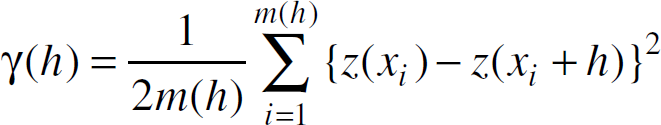
where m(h) is the number of samples separated by the lag distance h.

Data in high dimensions might add complexity in modeling variograms. If data lie in a high dimensional space, variograms are computed first in different directions separately. If variograms in different directions turn out to be more or less the same, the data under study can be assumed to be isotropic, then sample variograms are averaged together. Otherwise, data in different directions need to be modeled separately.

In Ordinary Kriging at unmonitored locations, the data is estimated as a weighted average of the neighboring samples,

Z (x_{0}) = \sum_{i = 1}^{N} λ_{i} z (x_{i})

(11)

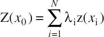
where $\sum_{i = 1}^{N} λ_{i} = 1$ .

There are various ways to determine the weights used in different spatial interpolation algorithms. In Kriging, the weights are determined by minimizing the estimation variance which is written as a function of the variogram,

v a r [\bar{Z (x_{0})}] = E [Z (x_{0}) - \bar{Z (x_{0})^{2}}] = 2 \sum_{i = 1}^{N} λ_{i} γ (x_{i}, x_{0}) - \sum_{i = 1}^{N} \sum_{j = 1}^{N} λ_{i} λ_{j} γ (x_{i}, x_{j})

(12)

where Γ(x_i, x_j) is the variogram value of Z between the sample points x_i and x_j, and Γ(x_i, x₀) is the variogram value of Z between the sample point x_i and the target data point x₀.

Minimizing the estimation variance (i.e., Equation 12) under the constraint that $\sum_{i = 1}^{N} λ_{i} = 1$ , (which is a necessary condition for an unbiased estimator) is a constrained optimization problem. It can be converted to an unconstrained optimization problem using the method of Lagrange multiplier. Specifically, a Lagrange parameter can be added to the Equation 12:

\begin{aligned} v a r [Z (x_{0}) = E [Z (x_{0}) - Z (x_{0})^{2}] \\ = 2 \sum_{i = 1}^{N} λ_{i} γ (x_{i}, x_{0}) - \sum_{i = 1}^{N} \sum_{j = 1}^{N} λ_{i} λ_{j} γ (x_{i}, x_{j}) - 2 μ (\sum_{i = 1}^{N} λ_{i} - 1) \end{aligned}

(13)

The unconstrained minimization problem expressed in Equation 13 can be solved by setting its partial derivative with respect to each δ_i and μ to be 0. It is a system of N + 1 of linear equations involving N − 1 unknowns and can be solved by methods for solving systems of linear equations, e.g., Gaussian Elimination or matrix inversions. The above linear equations can be rewritten in the matrix format as: Aλ=b, where

A = [\begin{matrix} γ (x_{1}, x_{1}) & γ (x_{1}, x_{1}) & \dots & γ (x_{1}, x_{N}) & 1 \\ γ (x_{2}, x_{1}) & γ (x_{2}, x_{2}) & \dots & γ (x_{2}, x_{N}) & 1 \\ ⋮ & ⋮ & \dots & ⋮ & ⋮ \\ γ (x_{N}, x_{1}) & γ (x_{N}, x_{2}) & \dots & γ (x_{N}, x_{N}) & 1 \\ 1 & 1 & \dots & 1 & 0 \end{matrix}]

(14)

b = [\begin{matrix} γ (x_{1}, x_{0}) \\ γ (x_{2}, x_{0}) \\ ⋮ \\ γ (x_{N}, x_{0}) \\ 1 \end{matrix}]

(15)

λ = [\begin{matrix} λ_{1} \\ λ_{2} \\ ⋮ \\ λ_{N} \\ μ \end{matrix}]

(16)

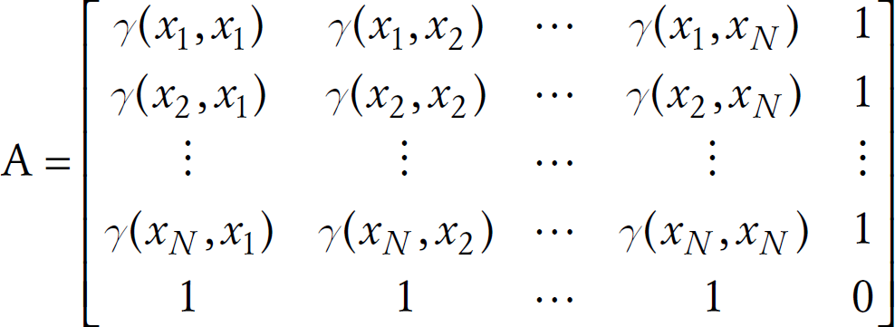
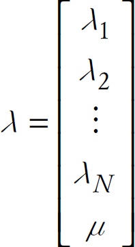
The weights and the Lagrange parameter can be obtained from

λ = A^{- 1} b .

(17)

Different interpolation techniques will generate multiple data sets from one single experimental data set. Which one is most desirable depended on the specific application and algorithm under study. For example, when we evaluate a wavelet compression algorithm [40], spatial correlation is identified as an essential data characteristic. We selected the synthetic data set that can best match the original experimental data in terms of its spatial correlation. Identifying a small set of parameters essential to the algorithm performance provided quantitative metrics that allowed us to directly evaluate the synthetic data sets.

Rather than suggesting one or optimizing one single interpolation algorithm for a single metric or specific type of data, we provided a suite of spatial interpolation algorithm implementations. A new spatial interpolation or synthetic data generation algorithm, e.g., the data generation technique proposed in [23], can be easily integrated into our scalable synthetic data generation framework.

4.1.2 Evaluation of synthetic data generation

Data Set Description and Spatial Interpolation Algorithms Implementation. We used the same set of S-Pol radar data (introduced in Section 2.1.1) in our evaluation.

We applied the afore-mentioned eight interpolation algorithms to the selected spatial radar data sets. We used the spatial package in R [2] to achieve Kriging. Nearest Neighbor, Bilinear, Bicubic, Spline interpolation results were obtained from the interp2() function in Matlab. Since Bilinear and Bicubic interpolation functions in Matlab provided no prediction for edge points, we used results from Nearest Neighbor interpolation for edge points in bilinear or bicubic interpolation results. Edge directed interpolation is from [12]. Inverse-distance-squared weighted average interpolation and Delaunay triangulation interpolation were implemented in Matlab following the interface of interp2().

Evaluation Metrics. The synthetic data is desired to closely approximate the experimental data. This can be examined in an indirect or direct manner. Comparing the algorithm performance using the experimental data and using the synthetic data was an indirect evaluation which will be discussed in Section 5. A visual comparison after plotting both synthetic data and experimental data is a direct evaluation. In this section, we focused on direct evaluation through quantitative metrics.

For our synthetic data generation, it is desirable that the synthetic data can closely capture the essential statistical features of the original data. The set of statistical features selected as evaluation metrics should be the important parameters that directly affect the algorithm performance. It is difficult to define a statistical feature set that is generally applicable to most algorithms and data sets. Instead, the evaluation metrics should be selected based on the application and algorithm under study. For example, a large percentage of existing data compression algorithms (including joint entropy coding and wavelet compression which is used in the DIMENSIONS system [17]) are sensitive to the spatial correlations in the data. In general, sensor networks are envisioned to be deployed in the physical environment and deal with data from the geometric world; we believe that many sensor network algorithms will exploit spatial correlation in the data. Therefore, we used spatial correlation of the synthetic data versus original data to assess the applicability of a synthetic data generation technique to the sensor network algorithm being evaluated.

In general, if a quantitative metric is defined for the identified data characteristics, the difference between this quantitative metric of the synthetic data and the original data is used as the evaluation metric for our synthetic data generation. In this section, we used variogram values to measure the spatial correlation in the data, and defined the evaluation metric for the synthetic data as follows: two data sets A and B (e.g., a synthetic data set and an experimental data set); their variogram values are denoted as {Γ₁, (h_i)} and {Γ₂ (h_i)} respectively where h_i) is sample separation distance between two observations; i=1, …, m. The Mean Squared Difference of variogram values of two data sets is defined as:

\sum_{i = 1}^{m} (γ_{1} (h_{i}) - γ_{2} (h_{i}))^{2} / m

Interpolation Resolution. We studied two extremes of interpolation resolutions:

Coarse grained interpolation: increase the interpolation resolution by 4. The coarse grained interpolation is used to evaluate how closely the synthetic data generated by different interpolation algorithms approximate the spatial correlation of the experimental data.

Fine grained interpolation. Starting with a radar data set with 1km spacing, we increased the resolution by 10 times in each dimension—resulting in a 590×590 grid with 100m spacing. Fine grained interpolation is an essential step in generating irregular topology data.

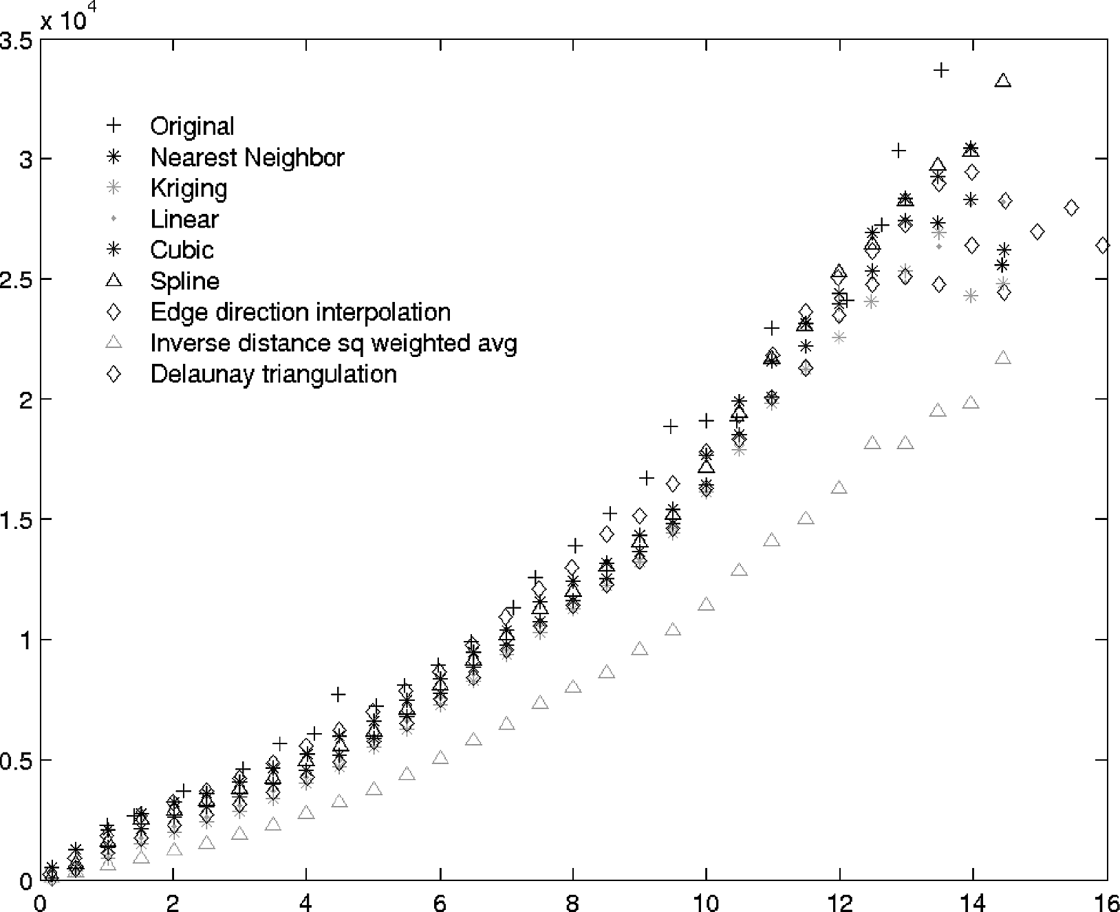
Evaluation Results. First, we visually presented the spatial correlation (i.e., variogram values) of the synthetic data in the case of coarse-grained interpolation. For the spatial dataset shown in Fig. 9, Fig. 10 shows the variogram plot of several synthetic data sets (generated from various interpolation algorithms) vs. the original data set. It demonstrated that the variogram curves of most synthetic data (except the one from Inverse-distance-squared weighted average interpolation) closely approximate the original one. At the long lag distances, the synthetic data may appear slightly under-estimating the long-range dependency in the original data. The source of this under-estimate may be caused by the smoothing effect of the interpolation algorithms.

FIGURE 9

Spatial modeling example: original data map. (60×60)

FIGURE 10

MSD of variogram values: Coarse grained interpolation results on a snapshot of radar data.

Further, we used the Mean Squared Difference between the variogram values of the original data and the synthetic data as a quantitative measure of how closely the synthetic data approximates the spatial correlation of the original data. Table 1 lists the Mean Squared Difference results averaged over 100 snapshots of radar data in increasing order. For the S-Pol radar data set (in both coarse grained interpolation and fine-grained interpolation), the Nearest Neighbor Interpolation matched best with the original variogram. In general most interpolation algorithms rank differently (relative to each other) in the case of fine-grained interpolation and coarse grained interpolation. We observed the same inconsistency with another precipitation data set [36]. In the case of fine-grained interpolation, we verified whether the spatial correlation in the synthetic data matched the experimental data at the extent of coarse granularity. At the scale of fine granularity, we do not have ground truth data.

TABLE 1

Mean Squared Difference of variogram values for different interpolation algorithms in the increasing order of MSD for coarse-grained interpolation

Name of method	MSD for coarse-grained interpolation
Nearest neighbor	8.354218e+01 (1.836358e+01)
Edge directed	1.970850e+02 (2.129320e+01)
Cubic	2.000790e+02 (1.694163e+01)
Delaunay triangulation	3.406270e+02 (4.795614e+01)
Linear	3.941510e+02 (2.876476e+01)
Spline	7.148526e+02 (5.5949e+01)
Kriging	1.469954e+03 (1.913371e+04)
Inverse-dist.-squared-weighted avg.	1.682726e+03 (3.617214e+02)

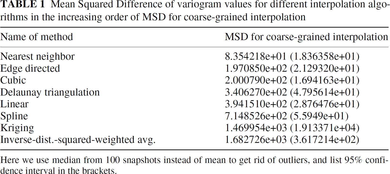
Here we use median from 100 snapshots instead of mean to get rid of outliers, and list 95% confidence interval in the brackets.

Based on these results, we do not recommend one single interpolation algorithm over others. We proposed to use spatial correlation as the evaluation metric for our synthetic data generation purpose and provided a suite of interpolation algorithms. Given a new synthetic data generation task, we would test with different interpolation algorithms selecting one that can best suit the algorithm and experimental data set under study. Although the Nearest Neighbor Interpolation appeared to be the best matching with the original variogram model, it is not appropriate in the case of ultra-fine grained interpolation; it assigns all nodes in a local neighborhood the same value from the nearby sample. Most physical phenomena have some degree of variation even in a small local neighborhood; therefore, we would not expect all sensors deployed in a local neighborhood report the same sensor readings as in the case of the nearest neighbor interpolation.

Summary. As shown above, most interpolation algorithms can approximate the original variogram models. However, it can only be used to interpolate at unsampled locations, not unsampled time. Furthermore, spatial interpolation algorithms, including Kriging, are not able to characterize the correlation between the spatial domain and temporal domain of the data such as variation of the time trend at each location and spatial correlation changes as time progresses. We wish to use the joint space-time model to address the limitations of the spatial interpolation techniques alone.

To generate synthetic spatio-temporal data, we started with an experimental data set which includes multiple snapshots recorded at various times. Inspired by a joint space-time model in [27], we modeled our data as a joint realization of a collection of space indexed time series, one for each spatial location. The coefficients of a time series model were space-dependent; we further spatially modeled them to capture these space-time interactions. Synthetic data are generated at both unmonitored time and location. This allowed us to generate synthetic data at arbitrary spatial and temporal configurations. Compared to applying spatial interpolation techniques to each snapshot of data separately, joint space-time modeling techniques allowed us to model the joint space-time dependency and variation in the data. In [40], we described this joint spatio-temporal model and presented our results on applying this model to the S-Pol radar data. In [40], we also discussed the trade-off between spatial interpolation and the joint space-time model. Even though the joint space-time model can capture the correlation between the temporal trend and spatial variation, it comes at a cost. When we compare the prediction accuracy of spatial interpolation to the joint space-time model at the same time instant, a spatial interpolation technique usually can capture data closer to the original than data from a joint space-time model.

4.1.3 Generating Synthetic Data in an Arbitrary Topology

In Section 4.1.1, we created a grid topology at a much finer granularity than our target topology. To generate a data set in an arbitrary topology, we overlayed the target topology on the ultra fine-grained grid data. Each node in the target topology is assigned a value from the nearest grid data. One could use interpolation techniques to directly generate synthetic data at an arbitrary location and time. However, providing an ultra fine-grained data set allows algorithm evaluations over the same underlying data correlation model but different topology settings.

4.2 Generating Synthetic Data Corresponding to a Wide Range of Parameters

When the experimental data covers a wide range of parameter values, it is sufficient to apply the techniques introduced above to generate synthetic data that can capture the original data features. However, if the existing experimental data from the relevant fields is scarce, the synthetic data generated from empirical models will have the same limited range as the experimental data. Thus, to address insufficient experimental data scenarios we designed algorithms to generate data sets corresponding to a wide range of parameter values.

For quantitative data metrics (e.g., data distribution, spatial correlation), we provided knobs to directly adjust these parameters. While for features that are difficult to characterize quantitatively, e.g., the spatial structure of the phenomena or the spatial distribution of data values, we provided test data suites that can cover a good percentage of parameter space.

As mentioned in Section 4.1.3, spatial correlation is an essential parameter to many sensor network algorithms. In [39], we proposed a synthetic data generation algorithm to directly adjust parameters in the spatial correlation model. The core idea of this data generation method is as follows. In the Kriging spatial interpolation process, the variogram values required in matrix 14 and 16 are derived directly from modeling the sample data sets. Alternatively, assigning Γ(x_i,x_j) and Γ(x_i,x₀) to a different value will generate synthetic data with a different spatial correlation feature from the experimental data. By varying the variogram values in Equations 14 and 16 across a wide range or using a different variogram model, we will be able to generate synthetic data with a broad range of spatial correlations. We refer readers to [39] for algorithm details. In [39], we demonstrated that by adjusting the variogram models based on a single experimental spatial data set we obtained synthetic data with a wide range of spatial correlations. This allowed algorithm evaluation against data corresponding to a wide range of spatial correlations.

As demonstrated in Section 2, data distribution is an essential characteristic to many statistics estimation problems. In [39], we proposed using stochastic simulation to generate data sets with adjustable data distribution characteristics. Due to space limitation, we leave out algorithm details here.

5. Algorithm Evaluation using our Synthetic Data

Our synthetic data generation toolbox can generate data in an arbitrary topology. A useful metric for these synthetic data is whether the synthetic data can capture important features of the experimental data or whether the synthetic data cover a wide range of parameter values in the dimension of interest to algorithms.

In Section 4.1.2, the synthetic data was evaluated directly in terms of the identified important parameters. Specifically, spatial correlation is identified as a feature essential to many sensor network algorithms. The Mean Squared Difference between the spatial correlation of the synthetic data and the experimental data is used as a quantitative metric for synthetic data evaluation. In this section, we evaluated the utility of the synthetic data through algorithm evaluation. The evaluation results confirmed the utilities of our synthetic data in the aspects of realistic data features and data spanning across a wide range of parameter values.

Algorithm Evaluation using Synthetic Data Across a Wide Range of Parameters: Median Computation by Random Sampling

As stated above, we recommend evaluating algorithms with data corresponding to a wide range of parameter values in order to identify the regimes in which the algorithm performs adequately. The parameter of interest could be data distribution, spatial correlation, or other data characteristics. The synthetic data generation techniques discussed in Section 4.2 can be used to generate realistic data sets corresponding to a wide range of parameter values.

We evaluated the median computation by uniform sampling algorithm discussed in Section 2.1.1 using synthetic data generated from the empirical models of the S-Pol radar data. Figure 11 (a) verifies that the median computation algorithm evaluated with our synthetic data exhibits similar behavior as that evaluated with the experimental data (Fig. 1(a)):

a strong correlation between the estimation accuracy and the corresponding p-percentile bin size in the data and

the algorithm performance demonstrated a wide range under various data input.

In addition, our synthetic data covered a similar range of data distribution as that of the experimental data.

FIGURE 11

Evaluation results using synthetic data generated from the radar data: the algorithm exhibits similar behavior as the evaluation results using the experimental data.

Algorithm Evaluation using Synthetic Data with Realistic Data Features: Fidelity Driven Sampling

We also applied the same synthetic data used above to the Fidelity Driven Sampling algorithm. The evaluation results (Fig. 11(b)) provided similar insights as the evaluation using data collected from a lab environment (Fig. 5(d)). The results indicated that the MSE achieved by the Fidelity Driven Sampling is slightly higher than the Raster Scan; when evaluated with data simulated from simple models (Fig. 4), the MSE achieved by the Fidelity Driven Sampling is several orders of magnitudes smaller than the Raster Scan.

6. Related Work

Data Modeling Techniques in Environmental Science

In environmental science or geophysics, various data analysis techniques have been applied to extract interesting statistical features from the data or estimate sensor values at un-sampled or missing data points. To generate synthetic data that can capture interesting features of the experimental data, we borrowed heavily from geostatistics and spatial interpolation techniques. In particular, we explored Kriging and several non-stochastical interpolation techniques. The joint space-time model used in our data analysis is inspired by and simplified from a joint space-time model proposed by Kyriakidis et al. [27].

Data Modeling in Database and Data Mining

Theodoridis et al. [34] proposed to generate spatio-temporal datasets according to parametric models and user-defined parameters. Since the parameter space is huge, it is impossible to exhaustively search the entire parameter space. Instead, we propose to start with an experimental data set and generate synthetic data that share similar statistics with the experimental data. DuMouchel et al. [35] proposed data squashing techniques to shrink a large data set to a manageable size. Although sharing the same objective of deriving synthetic data from modeling existing data, they considered non-spatio-temporal data. They assumed that a data set is the result of N independent draws from the same probability model. Often spatial and temporal stationarity do not hold for an arbitrary physical random process. As a result, the spatio-temporal data cannot be assumed to be drawn from the same probability model as assumed by [35].

TCP Traffic Modeling in the Internet

In the context of the Internet, researchers have studied TCP traffic modeling. For example, Caceres et al. [7] characterized and built empirical models of wide area network applications. The specific data modeling technique in their study [7] may not be able to capture a highly dynamical physical environment in which sensor networks are deployed, due to the following:

Sensor networks are closely coupled with the physical world; therefore, data modeling in sensor networks needs to capture the spatial and temporal correlation in a highly dynamic physical environment;

the characteristics of wide area TCP traffic are potentially very different from the workload or traffic in sensor networks.

Internet TCP traffic is the superposition of many TCP connections. However, sensor networks tend to be specially designed and used for one or a few applications. Sensor network traffic is triggered often by physical phenomena and the deployed signal processing algorithm.

System Components Modeling in Wireless Ad-hoc and Sensor Networks

Previous research has been carried out on modeling system components in wireless ad-hoc and sensor networks; however, most existing research focused on modeling communication channels ([25, 9, 42, 38]) and mobility models ([6, 10, 24]).

Ns-2[3] and GloMoSim [41] provided flexibility in simulating various layers of wired networks or wireless ad-hoc networks. However, they do not capture many important aspects of sensor networks such as sensor models or channel models. In contrast, Sensorsim [29, 30] directly targeted sensor networks. They introduced the notion of a sensor stack and sensing channel. Their work mainly focused on point source sensor models and exponential channel loss models. These models may capture point source phenomena, such as contaminant transport monitoring; however, it is not applicable to environmental phenomena in general. Our work could be used as a new model in Sensorsim.

Proposal on Better Input Models in the Context of the Internet

In the context of Internet research, Floyd et al. [14] illustrated the problems caused by inappropriate models. Although proposed in a different context, they shared similarity to our work in that both identified the significant influence that input models have on the algorithm performance; both proposed to use empirical models to guide the simulation to focus on scenarios representative of real world situations. Our work differed from theirs in the following two aspects: First, we modeled different subjects: they proposed to model topology and traffic mix patterns in an Internet application; we modeled sensor data input in a sensor network system. Consequently, their modeling techniques will not apply to sensor network contexts. Second, identifying a small number of parameters essential to the algorithm performance defined a unique feature of our system: a scalable synthetic data generation framework.

Synthetic Data Generation in Sensor Networks

The work in [23] proposed a mathematical model to capture the spatial correlation in sensor network data and to generate large synthetic traces from a small experimental trace. This synthetic data generation technique can be incorporated into our proposed synthetic data generation framework. However, as pointed out in [40], we lack ground truth data to verify that the large synthetic data traces match the statistics of the experimental data at fine scales. We do not recommend using models derived from a few sensor nodes to generate a large trace of fine granularity unless the phenomena is known to be smooth at small scales.

7. Discussion on Usage Models and Conclusion

In summary our proposed systematic evaluation methodology will help to identify the data features (i.e., parameters) that are important to an algorithm. Our synthetic data generation toolbox will provide data that can either capture the important features of the experimental data, or cover a wide range of parameter values in the dimension of interest to an algorithm.

Since data from different application domains or different sensing modalities may dramatically differ from each other, we need to address whether our proposed synthetic data generation framework is applicable to a different type of application or dataset. Even though a particular synthetic data set or a synthetic data generation algorithm may not apply to all sensor network algorithms, our proposed synthetic data generation framework is generally applicable. In some cases, certain synthetic data generation algorithms and the corresponding synthetic data generated therefrom may apply to multiple algorithms in the same application category. This occurs where those algorithms often share the same goal and exploit similar data characteristics for efficient communication.

In deploying sensor network systems, the functioning of these systems relies on that data characteristics assumed by the algorithm match the experimental data characteristics. To avoid an unpleasant surprise from simulation to deployments and ensure a robust algorithm design, the following guidelines in evaluating a new sensor network algorithm are recommended.

First, we evaluated the algorithm with some existing data. The initial data could be collected from remote sensing or other in-situ instrumentation. Employing the systematic performance evaluation techniques introduced in Sections 2 and 3, we identified the set of data characteristics essential to the algorithm performance. The challenge of the systematic evaluation is to identify the set of data characteristics that best defines the data dependency for a given algorithm. For example, these important characteristics could be data distribution or spatial correlation in the data. In general, identifying the relevant set of data characteristics will require a fair understanding of the algorithm under evaluation. The statistical analysis techniques are used to verify whether there is a strong correlation between the identified data feature and the algorithm performance.

Next, based on those identified essential data features, our synthetic data generation toolbox will generate data that can capture important features of real world phenomena and can accommodate flexible topology configurations. If the available experimental data is scarce, synthetic data can be generated corresponding to a wide range of parameter values along a dimension important to the algorithm. Evaluating algorithms using realistic data will help to validate that the range of parameter values in which the algorithm performed well matches real data characteristics in the deployment. In the case where the data characteristics assumed by an algorithm do not match the real data characteristics, the systematic evaluation recommended above will help identify the problem early and improve the algorithm design before deployments. Even with reliable remote code updating techniques available, in many cases, the events that the sensor networks are deployed to capture are not repeatable; therefore, it is important to ensure that an algorithm will work well before deployment.

Footnotes

1

If the estimation error metric is defined in terms of order (i.e., let p denote the real position of the estimated median $\overset{ˇ}{M} (Z)$ in the original data set, n/2 is the position of the real median, the estimation error is then defined as p-n/2). We prove ([]) that median computation by uniform sampling is not sensitive to data distribution. Intuitively, uniform sampling is applied in the spatial dimension. When the error metric is defined in the same dimension, i.e., position in an ordered list or space, the estimation error will not be sensitive to the underlying data distribution.

2

S-Pol (S band polar metric radar) data were collected during the International H2O Project (IHOP; Principal Investigators: D. Parsons, T. Weckwerth, et al.). S-Pol is fielded by the Atmospheric Technology Division of the National Center for Atmospheric Research. We acknowledge NCAR and its sponsor, the National Science Foundation, for provision of the S-Pol data set.

3

Briefly, [13] devised a method to transform ρ to a quantity z: (2)

z = \frac{1}{2} [l n (1 + ρ) - l n (l - p)]

z is distributed almost normally, independent of the sample size, with standard error approximately

σ_{z} = \frac{1}{\sqrt{n - 3}}

. The confidence interval for ρ can be derived from the confidence interval of a normally distributed z and

References

Locfit: Local regression and likelihood. http://cm.bell-labs.com/cm/ms/departments/sia/project/locfit/.

The r project for statistical computing. In http://www.R-project.org/.

Bajaj

Sandeep

Breslau

Lee

Estrin

Deborah

Fall

Kevin

Floyd

Sally

Haldar

Padma

Handley

Mark

Helmy

Ahmed

Heidemann

John

Huang

Polly

Kumar

Satish

McCanne

Steven

Rejaie

Reza

Sharma

Puneet

Varadhan

Kannan

Haobo

, and Zappala

Daniel

, “Improving simulation for network research,” Tech. Report 99–702b, University of Southern California, March 1999. Revised September 1999, to appear in IEEE Computer.

Batalin

M. A.

Rahimi

Liu

Kansal

Sukhatme

G. S.

Kaiser

W. J.

Hansen

Pottie

G. J.

Srivastava

, and Estrin

, “Towards event-aware adaptive sampling using static and mobile nodes,” Tech. Report 38, UCLA/CENS.

Beferull-Lozano

Konsbruck

Robert

, and Vetterli

Martin

, “Rate-distortion problem for physics based distributed sensing,” in IPSN, 2004.

Broch

Maltz

D. A.

Johnson

D. B.

Y.-C.

, and Jetcheva

, “A performance comparison of multi-hop wireless ad-hoc network routing protocols,” in Proceedings of the Fourth Annual ACM/IEEE International Conference on Mobile Computing and Networking (Mobicom'98), Dallas, TX, 1998.

Caceres

Ramon

Danzig

Peter B.

Jamin

Sugih

, and Mitzel

Danny J.

, “Characteristics of wide-area tcp/ip conversations,” In SIGCOMM. ACM, 1991.

Carmo

Manfredo Do

. Differential Geometry of Curves and Surfaces. Prentice-Hall, Inc., 1976, pp. 141–146.

Cerpa

Alberto

Wong

Jennifer L.

Kuang

Louane

Potkonjak

Miodrag

, and Estrin

Deborah

, “Statistical model of lossy links in wireless sensor networks,” Tech. Report 41, CENS, April 2004.

10.

Das

Samir R.

Perkins

Charles E.

, and Royer

Elizabeth M.

, “Performance comparison of two on-demand routing protocols for ad hoc networks,” in INFOCOM, Israel, March 2000.

11.

Delouille

Ronique

Neelamani

Ramesh

, and Baraniuk

Richard

, “Robust distributed estimation in sensor networks using the embedded polygons algorithm,” in Proceedings of the Third International Symposium on Information Processing in Sensor Networks, ACM Press, 2004, pp. 405–413.

12.

Xin

, “New edge-directed interpolation,” in IEEE Trans. on Image Processing, Oct. 2001.

13.

Fisher

R. A.

, Metron, Volume 1. issue 3 1921.

14.

Floyd

Sally

and Kohler

Eddie

, “Internet research needs better models,” in 1st Workshop on Hot Topics in Networks (HotNets-I), Oct 2002.

15.

The R Foundation for Statistical Computing . “The r project for statistical computing,” http://cran.stat.ucla.edu/, 1999.

16.

Ganesan

Deepak

Cristescu

Rzvan

, and Beferull-Lozano

Baltasar

, “Power-efficient sensor placement and transmission structure for data gathering under distortion constraints,” in Proceedings of the Third International Symposium on Information Processing in Sensor Networks, ACM Press, 2004, pp. 142–150.

17.

Ganesan

Deepak

Estrin

Deborah

, and Heidemann

John

, “Dimensions: Why do we need a new data handling architecture for sensor networks?” in Proceedings of the First Workshop on Hot Topics in Networks (HotNets-I), Oct 2002.

18.

Gentle

J. E.

Hardle

, and Mori

, Handbook of Computational Statistics, Concetps and Methods. Springer-Verlag, 2004.

19.

Goovaerts

Pierre

, Geostatistics for Natural Resources Evaluation. Oxford University Press, Inc., 1997.

20.

Gray

, “The Gaussian and mean curvatures,” in Modern Differential Geometry of Curves and Surfaces with Mathematica, CRC Press, 1997, pages 373–380.

21.

Greenwald

M. B.

and Khanna

, “Power-conserving computation of order-statistics over sensor networks,” in 23rd ACM Symposium on Principles of Database Systems (PODS), 2004.

22.

Isaaks

Edward

and Srivastava

, In An Introduction to Applied Geostatistics. Oxford University Press, 1989.

23.

Jindal

Apoorva

and Psounis

Konstantinos

, “Modeling spatially-correlated sensor network data,” in SECON, 2004.

24.

Johansson

Per

Larsson

Tony

Hedman

Nicklas

Mielczarek

Bartosz

, and Degermark

Mikael

, “Scenario-based performance analysis of routing protocols for mobile ad-hoc networks,” in Proceedings of the ACM Mobicom, Seattle, Washington, 1999.

25.

Konrad

Almudena

Zhao

Ben Y.

Joseph

Anthony D.

, and Ludwig

Reiner

, “A markov-based channel model algorithm for wireless networks,” in Proceedings of Fourth ACM International Workshop on Modeling, Analysis and Simulation of Wireless and Mobile Systems, ACM MSWiM, July 2001.

26.

Kumar

Animesh

Ishwar

Prakash

, and Ramchandran

Kannan

, “On distributed sampling of smooth non-bandlimited fields,” in IPSN, 2004.

27.

Kyriakidis

P. C.

Miller

N. L.

, and Kim

, “A spatial time series framework for modeling daily precipitation at regional scales,” in 82nd Annual Meeting of the American Meteorological Society, January 2002.

28.

Nath

Suman

and Gibbons

Phillip

, “Synopsis diffusion for robust aggregation in sensor networks,” Tech. Report IRP-TR-03-08, Intel Research.

29.

Park

Savvides

, and Srivastava

M. B.

, “Sensorsim: A simulation framework for sensor networks,” in MSWiM. ACM, August 2000.

30.

Park

Savvides

, and Srivastava

M. B.

, “Simulating networks of wireless sensors,” in The 2001 Winter Simulation Conference. ACM, 2001.

31.

Rabbat

Michael

and Nowak

Robert

, “Distributed optimization in sensor networks,” in Proceedings of the Third International Symposium on Information Processing in Sensor Networks, ACM Press, 2004, pp. 20–27.

32.

Rahimi

Mohammad

Pon

Richard

Estrin

Deborah

Kaiser

William J.

Srivastava

Mani

, and Sukhatme

Gaurav S.

, “Adaptive sampling for environmental robotics,” in IEEE International Conference on Robotics and Automation, 2004.

33.

Snedecor

George W.

and Cochran

William G.

, in Statistical Methods. The Iowa State University Press, 1980.

34.

Theodoridis

and Nascimento

Mario

. Generating spatiotemporal data sets in the www. In SIGMOD Record 29 (3), 2000.

35.

DuMouchel

Volinsky

Johnson

Cortes

, and Pregibon

, “Squashing flat files flatter,” in Proceedings of KDD, 1999.

36.

Widmann

and Bretherton

, 50 km resolution daily preciptation for the Pacific Northwest, 1949–94, http://tao.atmos.washington.edu/datasets/widmann/.

37.

Willett

Rebecca

Martin

Aline

, and Nowak

Robert

, Backcasting: An adaptive approach to energy conservation in sensor networks. in IPSN, 2004.

38.

Woo

Alec

Tong

Terence

, and Culle

David

, Taming the underlying challenges of reliable multi-hop routing in sensor networks. in Sensys, 2003.

39.

Yan

, “Scalable, synthetic, sensor network data generation,” Ph.D. dissertation, UCLA, 2005.

40.

Yan

Ganesan

Deepak

Girod

Lewis

Estrin

Deborah

, and Govindan

Ramesh

, “Synthetic data generation to support irregular sampling in sensor networks,” In Geo Sensor Networks, Taylor and Francis Publishers, Oct 2003.

41.

Zeng

Xiang

Bagrodia

Rajive

, and Gerla

Mario

, “Glomosim: a library for parallel simulation of large-scale wireless networks,” in Proceedings of the 12th Workshop on Parallel and Distributed Simulations - PADS' 98, May 1998.

42.

Zhao

Jerry

and Govinda

Ramesh

, “Understanding packet delivery performance in dense wireless sensor networks,” in Sensys, 2003.

Two Case Studies on Data Sensitivity of Wireless Sensor Network Algorithms and our Proposal on Scalable,Synthetic Data Generation

Abstract

Keywords

1. Introduction

Organization of the Paper

2. Statistics Estimation Applications

2.1 Sensitivity of Algorithm Performance on Data and Identification of Essential Data Characteristics

2.1.1 Median Computation by Uniform Sampling

3.1 Evaluating Fidelity Driven Sampling with Simulated and Experimental Data

3.1.1 Evaluation Results on the Simulated Data

Definition 1 (Normal curvature)

Definition 2 (Principal curvature)

Definition 3 (Mean curvature)

Definition 4 (Total mean curvature)

4.1 Generating Irregular Topology Data from Empirical Models

4.1.1 Generating Fine-Grained Synthetic Data

4.2 Generating Synthetic Data Corresponding to a Wide Range of Parameters

5. Algorithm Evaluation using our Synthetic Data

Algorithm Evaluation using Synthetic Data Across a Wide Range of Parameters: Median Computation by Random Sampling

Algorithm Evaluation using Synthetic Data with Realistic Data Features: Fidelity Driven Sampling

Data Modeling Techniques in Environmental Science

Data Modeling in Database and Data Mining

TCP Traffic Modeling in the Internet

System Components Modeling in Wireless Ad-hoc and Sensor Networks

Proposal on Better Input Models in the Context of the Internet

Synthetic Data Generation in Sensor Networks

7. Discussion on Usage Models and Conclusion

Footnotes

1

2

3

References