
Abstract
A multi-layered algorithm is proposed that provides a scalable and adaptive method for handling data on a wireless sensor network. Statistical tests, local feedback, and global genetic style material exchange ensure limited resources such as battery and bandwidth which are used efficiently by manipulating data at the source and important features in the time series are not lost when compression needs to be made. The approach leads to a more ‘hands off’ implementation which is demonstrated by a real world oceanographic deployment of the system.
Keywords
Introduction
Wireless sensor networks are the subject of much research [1],[2],[3] and networks of devices are already being deployed [4]. Robust and efficient deployment of these networks will require as much hands-off configuration and management as possible, as the size of these networks increase beyond trial dimensions. Incorporating intelligence in a low cost device is an important requirement if the limited resources of these networks are to be used effectively. This paper proposes a hybrid algorithm that is shown to fulfill some of the important requirements.
Efficient monitoring of environmental conditions over time and space is an important and developing field in it's own right, but also serves as a useful test case for more heterogeneous pervasive networks[5]. Mobile phones, laptops, pdas, all have limited bandwidth and battery power but extensive functional capabilities, and getting the most out of these devices in an increasingly networked society is a primary goal of ICT research.
This paper discusses a specific environmental application, namely oceanographic monitoring, but the application has many generic features. The devices involved are geographically remote, difficult to access, in harsh conditions and use cheap ‘off the shelf’ components [3]. This means that the findings of this research can be reliably applied to a range of other applications.
Secoas
The key aims of the Self-Organizing Collegiate Sensor (SECOAS) Network Project [36] are to investigate a range of novel and emerging technologies needed to create self-organizing networks of microcontrollers, integrate the best ideas into a sensor network, and prove that the network can be used by scientists to meet the needs of a dynamic and challenging sensing application. The test site is an off-shore wind farm [7] where the impact of the structure is as yet unknown. This project aims to provide an alternative to traditional oceanographic monitoring techniques that involve large, expensive, stand alone monitoring stations. The alternative is an array of relatively cheap, wireless devices that, while individually less powerful, can together characterize an area and share data locally to provide a more complete picture of oceanographic variable over time.
Like all wireless sensor network systems resources such as battery power will be limited in the SECOAS project [8],[9]. Analog to digital converters, microchips and radio equipment all use battery power, so the usefulness of every reading needs to be assessed on the node, to save resource expensive transmission.
Algorithm
The ‘algorithm’ is in fact a hybrid of several decision making and data handling systems. For the purposes of this paper we will assume that the data being handled has passed through some initial pre-processing. For example, tidal flow can be measured by averaging a number of tilt readings over time. Conventional measurement standards regarding the number of tilt reading that need to be gathered over a time period convert ‘tilt readings’ into a single ‘flow’ measurement. There are therefore 3 decision making components:
Sliding Window averaging – We can scan a temporal ‘Sliding Window’ of readings for sufficient deletion conditions. Given a time-series of sensor readings at t0, t1, t2 a simple analysis of the reading at t1 can decide how useful it is. If the reading at t1 is the average of the readings at t0 and t2 then its deletion will make no effect on the characterization of a time series, given that it's value can be interpolated from readings at t0 and t2. A deviation from the average by a small amount may also be acceptable if improved compression is required. A trade off between loss of information and compression must be made. So if t0 = 8 and t2 = 10 and we have an allowable ‘difference from average’ of 50% any value between 8.5 and 9.5 can be deleted. If we are worried about losing too many sequential values we can preserve any value that is subsequent to a deleted one but this will obviously reduce compression to a maximum of 50%. Local Rules – Internal condition monitoring that affects the frequency of some actions, using negative feedback to obtain a homeostatic behavior. A node may carry out none, one or many actions during a specific time period. Actions such as sensing, forwarding, and queue management. Each action has a cost in terms of queue occupancy, battery usage and bandwidth usage. By monitoring the condition of these resources the probability of carrying out these actions can be modified. For instance, if the queue length is near it's maximum it would be prudent to take fewer readings and/or to do more forwarding or if the battery is being used at an unsustainable rate, higher battery usage behaviors should be reduced and lower usage ones increased. We term this ‘local learning’. Parameter Evolution – A genetic style transfer and fitness based evaluation of internal parameters can enable nodes that are performing well to share their configuration with nodes that are performing less well. Methods 1 and 2 both involve several parameters, values that effect the performance (e.g. Reading at T1 is deleted if + or – Z% of the average of Reading T0,T2. Sensing probability is reduced by X if queue is above Y). Effective values for these parameters are discovered in advance using multi-parameter optimisation on a simulated environment. But this can only be as good as the simulated environment. By encoding these parameters in a genetic fashion the performance of the nodes can be evaluated and the genetic material for the ‘fittest’ nodes can be spread, while the genetic makeup of the less fit nodes is modified or dies out. The authors have previously explored this area in the very different embodiment of Active Networks [10],[11]
These approaches can be used separately or combined. (Figure 1). Results on real datasets are presented in the next chapter.

In situ data management schematic
Initially, a singly buoy was deployed that gathered 7 days of data for 6 channels at 10 minute intervals (Figure 2). The 6 channels were Electrical Conductivity (mS), Temp ('C), Water depth (m), Turbidity (g/l), Tilt 1 (mV) and Tilt 2 (mV). Due to hardware limitation only the first 3 values will be processed using this approach, the other 3 will be saved directly to a logger. Further details of the hardware and software installation are available elsewhere [3,10]

Buoy deployment off scroby sands
It is important to evaluate how much impact each step of the algorithm has so we will evaluate each element in isolation before looking at how the elements perform when combined.
If we look at a sliding window deletion approach we see that as we increase the range at which the middle value is deemed interpolate-able we get increased compression, but that this varies with each dataset. (Figure 3). There are more complex algorithms to decide if to delete the middle value of 3 (for instance, using standard deviations of longer time sequences) but this will suffice as a simple first approach. Simplicity is important for transparency but also because the PIC microcontrollers [13] used for this deployment are not powerful number crunchers and doing advanced floating point statistics would be stretching their capabilities too far. Temperature is the least varying reading, with similar values being recorded frequently. Water depth is far more variant and unpredictable so the sliding window approach is unable to remove as many water depth readings safely.
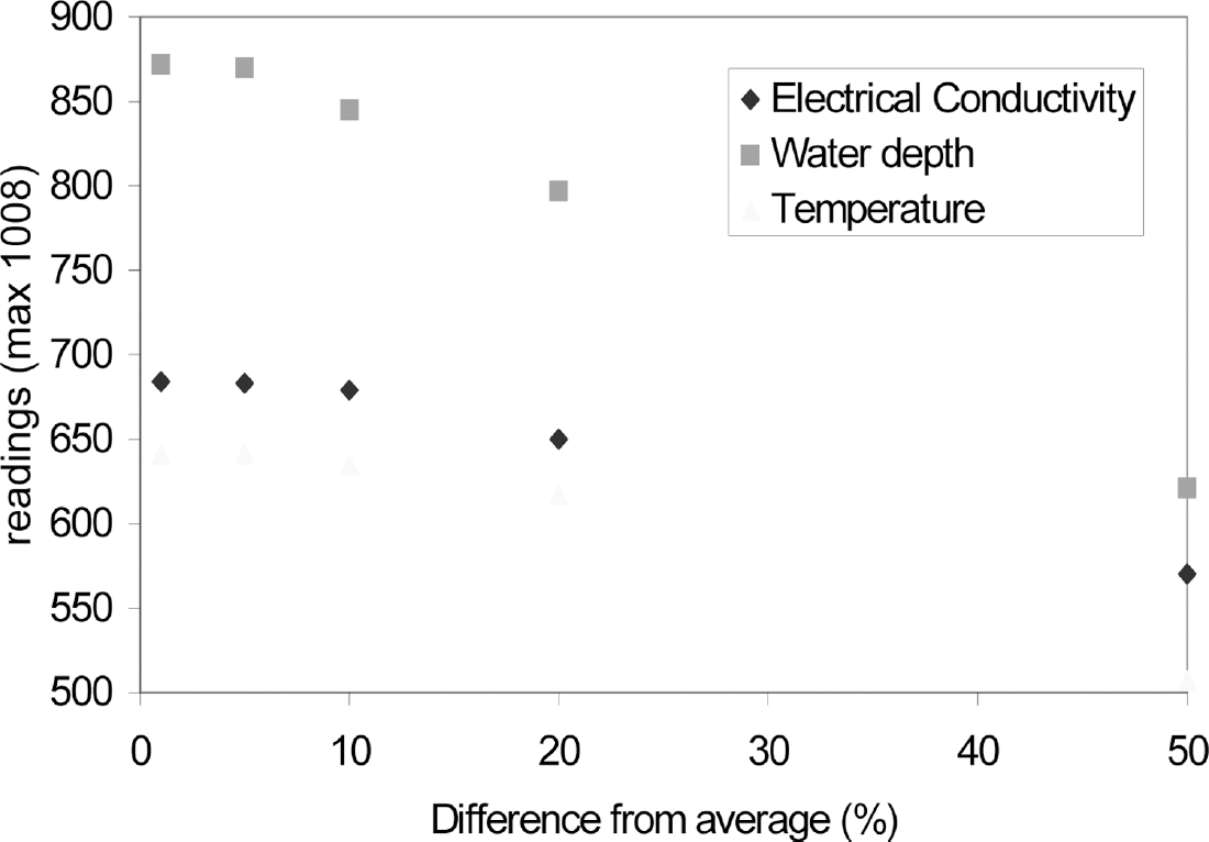
Deleting values that can be interpolated
Figure 4 shows how well the time series is characterized at increased compression rates. Deleted values are re-synthesized by taking the average of the previous and the subsequent point, the actual error is then calculated by referring to the original deleted value. For instance we might have three sequential depth readings at 10 minute intervals of 8.35, 8.525, 8.75metres. With a ‘difference from average’ value of 50% the middle value will be deemed deletable, when the resulting gap in the series is re-synthesized by averaging the previous subsequent values an interpolated value of 8.55 is generated, this deletion has therefore given rise to an error of 0.025 metres. This is a simple method of estimating missing values more complex ones may give rise to better approximations. An ‘allowable difference’ of 50% causes 38.4% of readings to be deleted and an error of 13.45 metres to be introduced, while an ‘allowable difference’ of 1% causes 13.5% of readings to be deleted and introduces an error of 4.32 metres over the 1008 measurements (about 0.043 cms per reading, when the average reading at 9.13 metres)

Characterization effectiveness with increased compression
Figure 5 shows how preserving any reading that follows a deleted one reduces compression. This in turn increases the quality of the characterization. Whether this is desirable will depend on the precise nature of the time series, deciding when how much freedom to give this component based on the nature of the readings is the subject of further research.

Difference in sliding window compression with and without preserving readings used to make deletion decision
The local learning component of the algorithm is more adaptive and is acting on different information, it is not interested in the values themselves but on the effect that making and forwarding readings is having on the condition of the node. Figures 6 and 7 show how the probability of 4 actions (sense, forward, compress, delete) adapt and stabilize over time. Figure 6 shows a node that has ample battery and bandwidth and as such can ‘afford’ to sense nearly every possible reading and forward elements in it's queue at a high rate. Less than one percent of readings are deleted or compressed. Figure 7 shows a node that is far more stressed, it has insufficient battery to sense and forward every possible reading. Here less than 30% of the possible number of readings are sent and many of these are compressed values made up of the average of 2 or more readings. The strength of this approach is that concrete knowledge of battery usage and bandwidth availability are not needed in advance of the experiment, these factors are heavily effected by environmental conditions so any estimates usually have to be conservative. If conditions for the experiment are unusually good then a non-adaptive approach would not be able to make use of the unforeseen excess in resources; conversely, if conditions were unusually bad, a non-adaptive approach may use the scare resources too liberally at the initial phases of the experiment thereby leaving no resources for the final stages. An adaptive approach, such as the one proposed, copes well in both scenarios adapting its behavior accordingly.

Action probabilities over time for a node with ample battery

Action probabilities over time for a node with limited battery power
A “quality of service” (QoS) measurement is included with every channel, this is defined by the user who deems a reading type (temp, conductivity, depth) to be of high, medium, or low importance. The delete function acts on members of the queue in a less severe manner if the reading is deemed a high importance reading. The QoS value is also modified by the local learning algorithm 1 (Figure 8).

User defined QoS values being self modified by analysis of variability of the associated readings
We can see in Figure 9 that as the network gets more bandwidth and become less stressed the success rate of returning readings increases, but when the network is under stress the low priority readings are dropped at a disproportionately high rate. This is a desirable feature as the user has already implied that if readings have to be dropped then he would prefer the low priority reading to be dropped preferentially.

Effect of QoS priorities in stressed network
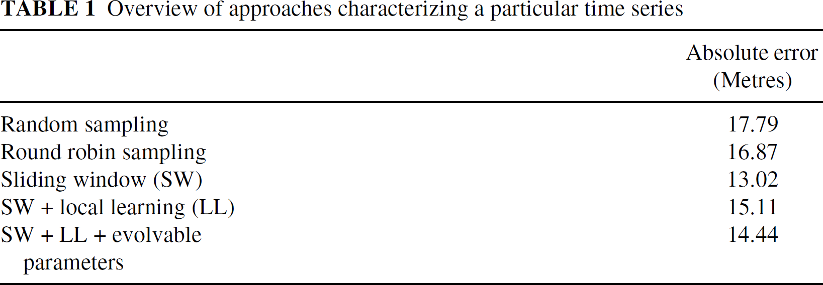
Overview of approaches characterizing a particular time series
The parameter evolution component is only tentatively examined. A simulation of 6 nodes was carried out with them sharing probability values (Pvalues) for the 4 actions (sense, delete, compress, and forward). Sense actually takes a value from the logger, forward sends half of the current queue to the base station, compress averages 2 points into one and delete removes a vale from the queue. Fitness rewards and penalties were given for a range of behaviors (penalties for attempting to forward items when the queue was short, for deleting high QoS items. Rewards for forwarding high QoS packets, for keeping battery usage within a desired range etc). By the end of a simulation, nodes sharing Pvalues managed to send, on average, 5% more readings over the same time period with the same battery as nodes not using parameter evolution. The effects of parameter evolution need to be further examined as performance is a more complex function than just the number of readings sent. Characterizing the performance of this sensor network will be the subject of another paper.
As one final overview we looked at how well different approaches characterized a particular time series. The methods used were Random, Round Robin, Sliding Window(SW), Sliding Window + Local Learning (LL) and Siding Window + Local Learning + Evolvable Parameters. All methods were configured to compress 1008 readings (10 minutely measurements for water depth over 7 days) by about 50%, to about 500 readings. Round Robin sampling is most like conventional sampling approaches, where a priori battery usage estimates may indicate that only 1 in 2 readings can be taken 2 .
While these are simplistic measurements it still shows that the approaches detailed in this paper offer powerful, ‘hands off’ solutions for intelligent data gathering and forwarding when compared with less intelligent and adaptive methods. The simple sliding window approach clearly offers a better in situ compression. Lesser improvements are offered by the more hybrid approaches over straightforward sampling methods, but the real time adaptability offered by reacting to internal and external conditions would not show up in this statistic. The ability to react to unforeseen circumstances is more difficult to measure but no less important. Evolvable parameters have more of an impact over longer time periods and, as in the real world, are more effective with bigger population sizes. Figure 10 shows a short snapshot of the sea depth, it is apparent that the full algorithm is sampling in an efficient and adaptive manner given the battery limitations.

Effectiveness of the SW + LL + evolvable parameters approach for data management on a restrictive power budget
Recording and characterizing a selection of time dependent environmental readings is made more complex if the resources to do this are limited. Given limitless resources every possible reading could be sent back to the base station and computationally intensive analysis could be carried out there. For the SECOAS project the limited resources include battery power, bandwidth and processor limitations. If we want to avoid a regimented protocol full of rules based on, as yet, unknown behaviors and conditions, we need an adaptive, intelligent approach that uses resources effectively. An approach that can decide if a measurement is useful before it is sent on its costly journey to a base station. That can adapt to changing circumstance that were unforeseen at the beginning of the experiment. That can juggle with user requirements, hardware constraints, and reading variability to produce as good a set of measurements as possible.
The algorithm presented in this paper is made up of several layers of simple actions. Simple short-range analysis of 3 values enables the most redundant values to be dropped at the source, homeostatic local loops enable actions to be carried out in a sustainable manner, and evolutionary structures enable successful nodes to share their ‘knowledge’. The individual components need to be simple and tractable if they are to be successful on a low power, low cost device but the end result of the layering of these components is powerful enough to enable much deeper characterization of environmental conditions than would be traditionally possible. This type of ‘hands off’ management is still in it infancy but its successful application will enable the wireless sensor networks to fulfill their undoubted promise and may in turn lead to much more use being made of increasingly pervasive and networked computational devices of all kinds.
Footnotes
1
A running measure of variance is kept and if recent variance is higher than long term variance the QoS value is increased and vice versa.
2
This is a fairly modest compression, it is safe to say that as compression requirements increase the importance of more intelligent compression algorithms detailed in this paper also increases.