Sage Journals: Discover world-class research

Abstract

We present a rigorous geometric analysis of the computation of the global positions of an airborne video camera and ground based objects using aerial images of known landmarks. This has also been known as the perspective-n-point (PnP) problem. A robust Hough transform-like method, facilitated by a class of CORDIC-structured computations is developed to find the camera position followed by a method of computing the position of a ground object from images of that object and three known landmarks. The results enable fast and effective visual terrain navigation of aerial surveillance systems when the global positioning and inertial navigation sensors become faulty, inaccurate, or dysfunctional. These new hardware implementable algorithms can also be used with MEMS based INS sensors through a multisensory fusion process.

Keywords

Visual Navigation GPS Fault Tolerance Unmanned Air Vehicles Low-altitude Aerial Imagery

I. Introduction

In terrain navigation, the global position of an airborne camera system and its orientation are usually measured through onboard GPS and INS sensors. However, there are circumstances where the position and direction given by the GPS and INS sensors are not accurate due to built-in errors, poor signal to noise ratio, intentional R-F jamming, or faulty operation of the sensors. In such cases, video images of known landmarks can be used to perform visual navigation, hence compensate the GPS and INS errors and dysfunctions [1] [2].

The perspective-n-point problem deals with determining the global position of the camera from images of known landmarks, given the intrinsic parameters of the camera. In case there are three non colinear landmarks, a set of three quadratic equations with three unknowns can be formed [3], that can produce as many as eight solutions. Fischler and Bolles [4] derive a biquadratic polynomial equation with one unknown, that has a maximum of four solutions. For the case of four landmarks, Rives et al. [3] find a unique solution if the landmarks are coplanar by finding the solutions using three landmarks, then verifying them with the fourth one. If the four landmarks are not coplanar, they derive a set of six quadratic equations with four unknowns. Horaud et al. [5] form a biquadratic polynomial equation in one unknown for non-coplanar landmarks. The equation can have as many as four solutions, but some of them can be eliminated. A more general approach to finding solutions for the PnP problem is to use the least-square techniques [6].

We present our analysis for the problem through constructive geometry. The main result of the analysis is: for any two landmarks in an image, we can construct a unique toroid in the world space, that constitutes all possible positions of the camera [7]. The toroid can be easily generated using a CORDIC [9] structured hardware, to register a vote at the appropriate cells of a three-dimensional array of accumulators. For example, in the case of four landmarks, six toroids could be generated, corresponding to the six quadratic equations derived by Rives et al. [3]. An acceptable solution would be identifiable at the cell with a vote of at least three and at the most six. The geometric nature of the proposed approach helps understand the span of the subspace (3-dimensional world) to which the expected solution would be constrained. Thus, a finite number of accumulators are sufficient. Moreover, we use a multi-resolution recursive approach outlined in [10] for the implementation. That is our Hough transform-like method for locating the accurate position of the camera when there are more than two landmarks.

A task for an airborne camera system is to find the global positions of ground locations from their images taken by its camera. If the positions and directions of the camera during its flight are known, performing this task is fairly simple by adapting multiview reconstruction techniques for calibrated cameras to apply for a single moving camera. It is still possible to determine 3-D positions of points from their images taken by a moving camera even if camera direction is unknown. Roach and Aggarwal [11] showed that the positions of five points and camera motion can be recovered from their images in two frames by solving a set of 18 non-linear equations and used an iterative finite difference Levenberg-Marquardt algorithm to solve the equations.

There is a growing recognition and widespread demand for unmanned vehicles [12]. Substantial work is in progress [8] to make them inexpensive, easy to deploy and potentially expendable. These systems are envisioned to constitute a sophisticated sensor network in critical applications, where low altitude aerial imagery is both accessible and a requirement. Urban applications must be prepared to address potential vulnerabilities of on-board GPS devices due to EMI and intentional RF-jamming. The work reported here will be very valuable in such a sensor network.

In the context of terrain navigation with known landmarks, we present a closed-form solution to compute the positions of ground locations using as few as two image frames with a minimum number of three landmarks. The solution allows fast computations of 3-D positions from their images when INS is not available.

II. Imaging Model

The geometric model of the aerial imaging system is illustrated in Fig. 1. Perspective imaging model [13] is used. Notations used in this paper are as follows: Objects located at points A and B, whose coordinates in the 3-D world coordinate system are represented by vectors X _A = [X_AY_AZ_A]^T and X _B = [X_BY_BZ_B]^T, are imaged by a camera at C. Their coordinates in the camera-centered coordinate system are represented by X′ _A = [X′_AY′_AZ′_A]^T and X ′ _B = [X′_BY′_BZ′_B] ^T . The transformation from world coordinate system to camera-centered coordinate system is represented by a rotation matrix R and a translation vector t, such as:

X^{'} = R X + t

(1)

Figure 1

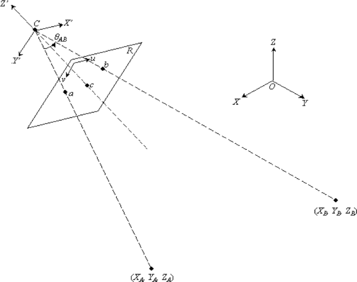
Two objects at A and B imaged by a camera at C. θ_AB is the angle subtended by line-segment AB, measured accurately at the image-resolution.

Image points a and b of objects A and B, respectively, are on the plane Z′ = −f, called the image plane, in the camera-centered coordinate system, where f is the focal length of the camera. Thus, x _a = [u_av_a]^T and x _b = [u_bv_b]^T represent the coordinates of a and b in the image plane. Let c denote the intersection between axis Z′ and the image plane. The point c is called the image center, whose image coordinates are given as: x₀ = [u₀v₀] ^T .

Lemma 1

The angle θ _AB = ∠ACB subtended by the 3-D line segment AB at the pupil of the camera C can be measured accurately without any explicit knowledge of the exact geoposition and orientation of the camera.

Proof. Assume that the video imaging system has already been calibrated, and its camera intrinsic parameters such as the location of the image center, pixel dimensions, and focal length have been determined and made available. Also, we assume that the exact locations of the points a and b have been determined by standard image processing techniques at the best possible accuracy. Thus, the 3-D coordinates of points a and b in the camera-centered coordinate system are given by:

X_{a}^{'} = - [\begin{matrix} (u_{a} - u_{0}) p_{u} \\ (v_{a} - v_{0}) p_{v} \\ f \end{matrix}]

(2)

and

X_{b}^{'} = - [\begin{matrix} (u_{b} - u_{0}) p_{u} \\ (v_{b} - v_{0}) p_{v} \\ f \end{matrix}]

(3)

where p_u and p_v are the intrinsic parameters defining the pixel size of the camera.

Let N _A and N _B be the unit normal vectors of two lines (C. A) and (C. B), respectively, in the camera-centered coordinate system. We have:

N_{A} = \frac{X_{a}^{'}}{| X_{a}^{'} |}

(4)

and

N_{B} = \frac{X_{b}^{'}}{| X_{b}^{'} |}

(5)

Then, the angle θ _AB can be computed as follows:

θ_{A B} = across (N_{A} ∙ N_{B})

(6)

Thus, the angle θ _AB can be measured indirectly from images of points A and B. Moreover, the differential nature of the quantity θ _AB makes it insensitive to the orientation jitters of the camera.

III. Finding Camera Position

A. Geometric Analysis

Our results are based on the classic theorem of angles on circles [14] which states: Given a circle and a chord AB dividing the circle into two sectors, the angle subtended by the line AB at the center is exactly twice that of the angle subtended by the are AB at any point on the circumference along the sector AB. Its corollary states that: the locus of the vertex C of all triangles with a fixed apex angle ∠ACB and fixed end point A and B is a sector of a circle [14].

Theorem 1

Given an image of two landmarks and therefore the angle subtended by them at the pupil of the camera, the unknown geoposition of the camera is constrained to a unique circle on the principal plane of imaging; and, it is also constrained onto the surface of a unique toroid in space when the principal plane can not be uniquely fixed.

Proof. We prove the above claim by constructing the circle and the toroid as described below.

Let the points A and B be the two landmarks observed by a camera at an unknown geolocation C. Then, the plane ACB is the principal plane as shown in Fig. 2. The angle θ _AB = θ can be measured from image, as shown in II. Also, let N _P be the unit normal vector of the principal plane ACB. And, let l be the length of the line segment AB. From the geolocations of A and B compute the midpoint M on AB. Draw the bisector of AB, the line perpendicular to AB passing through M. Locate the center I on the bisector at a distance h from M; and, compute the radius r as:

h = \frac{l}{2} \frac{1}{tan θ}

(7)

Figure 2

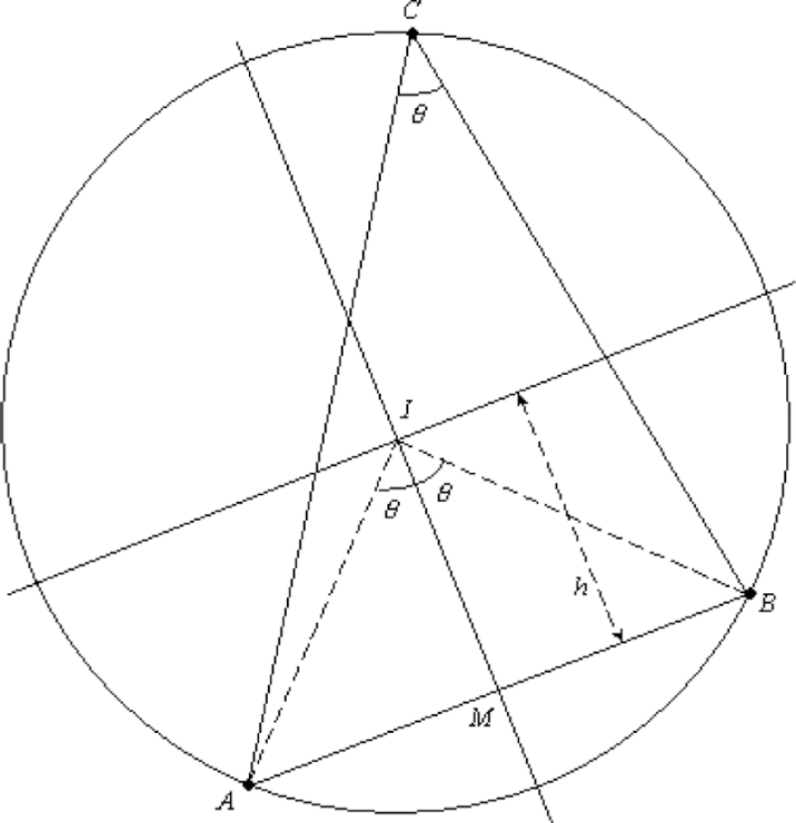
Two landmarks A and B are imaged from a camera at an unknown geolocation C. The angle θ_AB = θ is measured from the image. The circle constructed from two points A and B and the value θ is unique.

and

r = \sqrt{(h^{2} + \frac{l^{2}}{4})}

(8)

Also,

X_{M} = \frac{X_{A} + X_{B}}{2}

(9)

The unit normal vectors L of the line segment AB and P of its bisector are given by:

L = \frac{X_{B} - X_{A}}{| X_{B} - X_{A} |}

(10)

and

P = N_{P} \times L

(11)

Then, trace the locus of all possible positions of the camera C, by tracing X _C (α), (θ − π/2 ≤ α ≤ 3π / 2 − θ)

X_{C} (α) = X_{M} + h P + (r cos α) L + (r sin α) P .

(12)

Based on the Theorem of Thales [14], we can prove that the circle is unique.

When the principal plane is not explicitly known, any plane can be used to construct the circular are first, which is then rotated about the axis AB to create the toroidal surface. For example, consider the unit vector $E_{3} = (1 / \sqrt{3}) (1, 1, 1)$ . If L ≠ E₃ then let N _B = E₃; else, let $N_{B} = (1 / \sqrt{3}) (- 1, 1, 1)$ . Compute N _P = N _B × L, P = N _P × L, and Q = L × P. Then, for any (α,β) such that –π < β ≤ π and θ − π / 2 ≤ α ≤ 3π / 2 − θ, compute X _C (α,β) on the surface of the toroid as:

X_{C} (α, β) = (v_{α} cos β) P + (v_{α} sin β) Q + u_{α} L + X_{M}

(13)

where

u_{α} = r cos α

(14)

and

v_{α} = h + r sin α .

(15)

This completes our proof.

These computations follow a CORDIC structure; hence, they can be implemented in hardware [9] to rapidly generate the circle and the toroid. For example, the value of X _C (α) can be computed as follows, using a recursive algorithm:

α_{0} := 0; u_{0} := 1.0; v_{0} := 0;

(16)

[\begin{matrix} u_{k} \\ v_{k} \end{matrix}] = [\begin{matrix} 1 & δ \\ - δ & 1 \end{matrix}] [\begin{matrix} u_{k - 1} \\ v_{k - 1} \end{matrix}]

(17)

α_{k} = α_{k - 1} + δ

(18)

X_{C} (α_{k}) = X_{0} + h P + u_{k} L + v_{k} P

(19)

where δ ≍ sinδ is chosen as δ = 2⁻⁸, to perform the computation rapidly in hardware [9].

B. Hough Transform Approach

Hough transform [15] is a popular method to identify global patterns among a set of points in the image space. The basic idea of the Hough transform approach is:

Finding a way to parameterize the patterns of interest.

Mapping the points in the image space into the parameter space which is clustered so that a voting technique can be used to determine the most likely values of the parameters of the patterns appearing among the given set of points

As it is shown in the previous section, for every two landmark points in the image space, there is a unique toroid in the three-dimensional XYZ space, onto which the camera position is constrained. When there are more than two landmarks, it is likely that all of those toroids intersect at one point where the camera is located. Divide the XYZ space into a three-dimensional grid of accumulative cells, also called the Hough bins. To find the camera position in the grid, discretize all the toroids over the grid, then find the cell that has the highest number of votes. The discrete values of each toroidal surface can easily be generated by using the equations (13), (14), and (15) with the values of α and β incrementing from 0 to 2π.

A problem we have here is the space to be covered in the world coordinate system XYZ may be too large, that makes it impossible to use the clustering technique mentioned above to locate the camera position. Fortunately, in terrain navigation we have many ways to quickly estimate the proximity of the camera position, for examples,

from data provided by GPS with known maximum errors, or

from previous GPS data before the GPS becomes faulty, using some trajectory tracking method such as Kalman filtering to estimate the current position.

Hence, the search space can be limited into a relatively small volume for which the clustering technique is deemed effective. We also employ a multi-resolution approach to speed up the computation: using an iterative coarse-to-fine accumulation and search strategy [10].

Another problem that must be addressed arises due to the errors introduced by the discretization process. This problem needs special consideration in our case because the toroids are generated by incrementing the angles α and β, while the space is divided along the X, Y, and Z axes. A discussion of the problem, including how to select the incrementing procedure, and error analysis, is provided by Ballard in his paper on the generalization of Hough transform methods [16].

C. Special Configurations

There are special cases in which we can simplify the results of III-A so that faster computations can be achieved. The cases to be presented in this section are based on our observation that, if there are three colinear landmarks, then the camera position can be constrained to a unique circle in the world space.

Theorem 2

Given an image of three colinear landmarks, and the orientation of the principal plane of imaging, the geolocation the camera is uniquely determined.

Proof. Let L₁, L₂, and L₃ be the three landmarks. By definition, we know the orientation of the principal plane and three points on the plane, hence it is uniquely fixed. Two uniquely defined circles are constructed on the principal plane by applying Theorem 1, to the landmark pairs {L₁,L₂} and {L₂,L₃}, respectively.

Example. Consider an instance shown in Fig. 3, where the landmarks are located at (0,0), (2,0), and (2 + 2λ, 0) for some λ > 0 on the x-axis of the plane ACB. The pairwise differential angles subtended at the camera by the two consecutive pairs of landmarks are θ₁ and θ₂, respectively. Then, the camera position (x_c,y_c) in this plane can be uniquely extracted as:

(x_{c}, y_{c}) = (\frac{2 (1 - m β_{1})}{m^{2} + 1}, \frac{2 m (1 + β_{1})}{m^{2} + 1})

(20)

where, β₁ = cot θ₁, β₂ = cot θ₂, and m = (λβ₂ − β₁)/(1 + λ). In a more general case we assume the landmarks to be at (0,0), (d₂,0), and (d₃,0). Then, let λ = (d₃ − d₂)/d₂ and scale the final solution by a factor of d₂/2.

Figure 3

Three colinear landmarks in the most canonical and parameterized configuration and the uniquely found location C of the camera computed from θ₁ and θ₂ and λ.

Theorem 3

Given an image of three colinear landmarks, then the geolocation of the camera is constrained to a circle on a plane perpendicular to the line passing through the landmarks; and, both the circle and the plane are unique.

Proof. Let L₁, L₂ and L₃ be the landmarks; and let L be the direction cosine of the line x passing through these landmarks. Let N_P be the unit normal vector of a plane passing through the colinear landmarks. One such normal vector can be uniquely identified following the procedure used in the proof of Theorem 1. Also, P = N _P × L. We apply the insight gained from the canonical example above. Let d₂ and d₃ be the pairwise distances of the landmarks L₂ and L₃ from L₁, respectively. Then,

X_{C} = X_{L_{1}} + s x_{c} L + s y_{c} P

(21)

where s = d₂/2 is the scale factor for applying the results of the canonical results from the example. Now, rigidly rotate the entire plane around the axis x by 2π. It will produce a circle of radius sy_c contained in a plane perpendicular to x; and, the plane is at a distance sx_c from the landmark L₁. Since C is unique and x is fixed, both the circle and the plane of the circle are unique. Hence the claim.

Consider another special case where there are four coplanar landmarks, and no three colinear. We extend the result from Theorem 3 to show that, with these four coplanar landmarks, we can construct two circles in the world space. Note that these two circles can intersect at no more than two points, and in that case one of the intersections will be on or below the ground plane, as shown in Fig. 4. It means we can derive an analytic solution for the case of four coplanar landmarks from our constructions. However, in reality the inaccuracies introduced due to discrete sampling of the images with finite pixel size may result in a situation where these circles may not intersect. Obviously, our Hough transform-like approach provides a robust technique to accommodate that.

Figure 4

Four coplanar landmarks in a canonical configuration are imaged by a camera at C; two circles are computed from the two sets of diagonals of the quadrilateral ABMN. The chord of intersection of the circles, shown in a dotted line, is perpendicular to the ground plane.

We have also developed another method which extracts the camera position from the images of three landmarks. The formulation exploits another classic result on triangles, known as the Law of Sines, which states that: given a triangle, the ratio between the sine of each angle and the corresponding opposite-side is constant. The method is essentially a one-dimensional iterative search, modelled as a hypothesize and verify procedure, and has been experimentally verified to produce up to eight solutions.

IV. Finding Ground Locations

In this section we present a simple technique using known landmarks to compute geopositions of ground locations when INS is not available.

Lemma 2

Given the geoposition of a camera and of three non colinear landmarks and a fourth point whose position is unknown; then, the optical ray going through the optical center of the camera and the fourth point can be uniquely identified from a video image of all four points.

Proof. Let θ₁, θ₂ and θ₃ be the angles subtended at the camera between point G, whose position is unknown, and each of the three landmark points L₁, L₂, and L₃, respectively (Fig. 5). According to Lemma 1, these angles can be computed from images of four points captured by the camera. Let N₁, N₂, and N₃ be the unit normal vectors of the optical rays going through each of the landmark points. Because the geopositions of the camera and the landmarks are known, these normal vectors can be computed as follows:

N_{i} = \frac{X_{L_{1}} - X_{C}}{| X_{L_{1}} - X_{C} |} (i = 1, 2, 3)

(22)

Let N _G be the unit normal vector of the optical ray going through point G. We have:

N_{i} X_{G} = cos θ_{i} (i = 1, 2, 3)

(23)

[\begin{matrix} N_{1}^{T} \\ N_{2}^{T} \\ N_{3}^{T} \end{matrix}] N_{G} = [\begin{matrix} cos θ_{1} \\ cos θ_{2} \\ cos θ_{2} \end{matrix}]

(24)

Figure 5

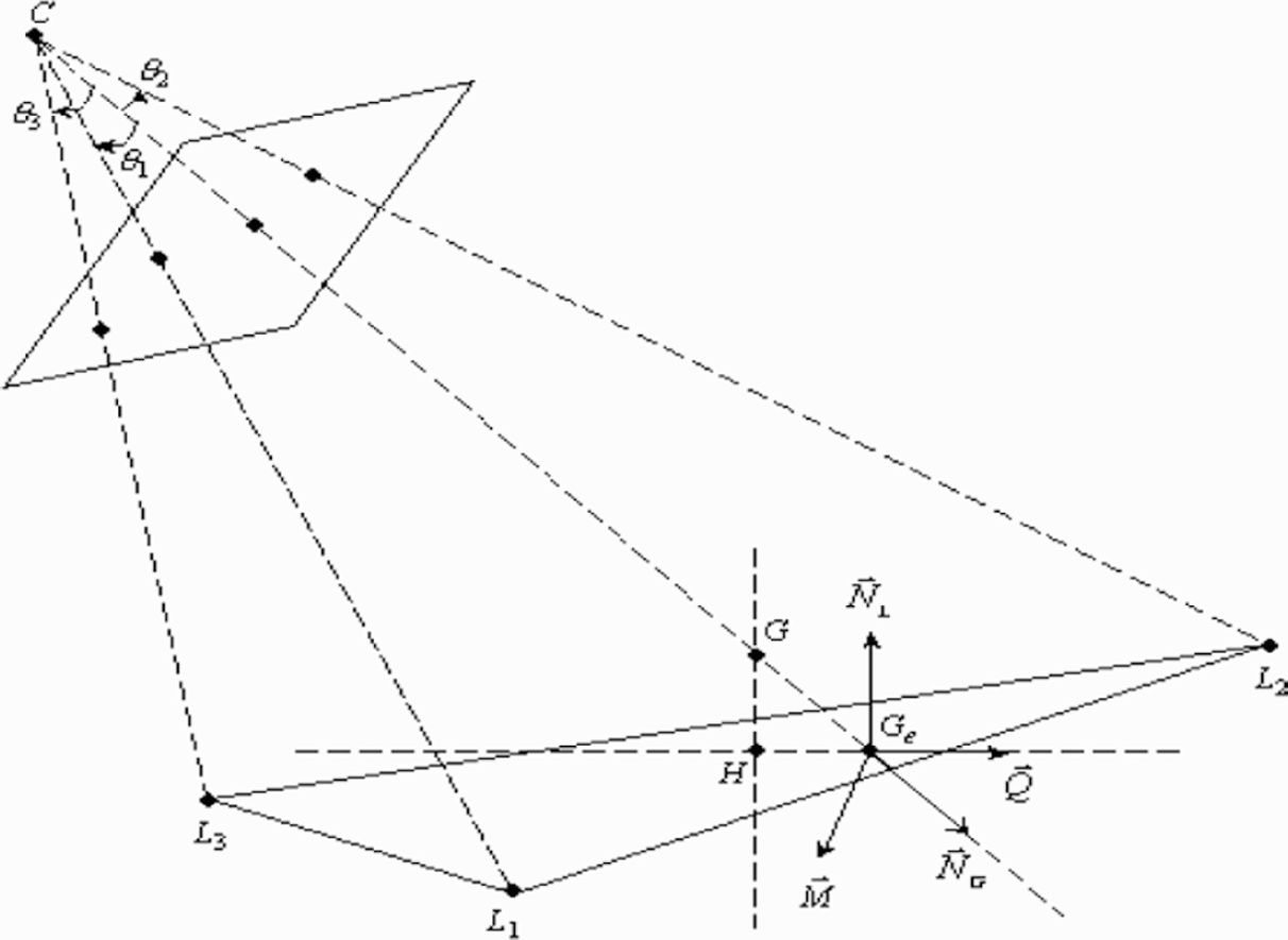
Four points are imaged by a camera located at C, in which L₁, L₂, and L₃ are known landmarks, and G is a point whose position is unknown. The ray (C, G) can be uniquely identified from θ₁, θ₂, and θ₃ measured from the images of four points.

that leads to the following formula to compute the normal vector N _G :

N_{G} = {[\begin{matrix} N_{1}^{T} \\ N_{2}^{T} \\ N_{3}^{T} \end{matrix}]}^{- 1} [\begin{matrix} cos θ_{1} \\ cos θ_{2} \\ cos θ_{2} \end{matrix}]

(25)

which is valid when four points C, L₁, L₂, and L₃ are non-coplanar. This completes our proof.

The geoposition of G can be computed from as few as two image frames acquired from an airborne camera. In each instance, a unique 3D line is to be found by applying the insights gained in the above lemma. In general a 3D point can be found at the intersection of two arbitrary lines which are not parallel or skewed. In practice, however, computational errors such as those caused by aliasing and discretization of measured image points cause the estimated lines to not intersect. To overcome that problem, we find the perpendicular projection H of G on the plane defined by three points L₁, L₂, and L₃ first, then calculate the distance from G to that plane, instead of computing the position of G directly.

It may not be so obvious as to why one should estimate the line passing through G and then solve for its geolocation, instead of applying standard stereo imaging principles directly on the images. The standard stereo computation would require precise measurement of change in orientation of the video cameras between the two instances of imaging all four points. The situation at hand is more constrained than an arbitrary stereo problem, in that, both the orientation and the location of the camera, in a limited sense, are bootstrapped from each video image of the three landmarks. This also explains why we are able to produce a closed form solution, for computing the location of G from two video images. Such a result is useful in low altitude imaging where, the on-board GPS is typically more accurate than the orientation sensor which are challenged due to wind turbulence.

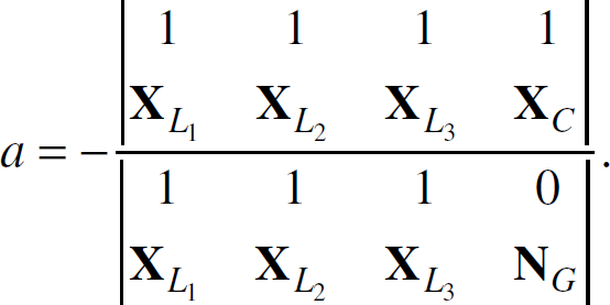
Let G_e be the intersection between the optical ray going through G and the plane (L₁,L₂,L₃), the coordinates of G_e in the world coordinate system can be computed as follows:

X_{G_{e}} = X_{C} + a N_{G}

(26)

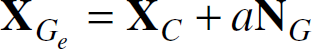
where

a = - \frac{| \begin{matrix} 1 & 1 & 1 & 1 \\ X_{L_{1}} & X_{L_{2}} & X_{L_{3}} & X_{C} \end{matrix} |}{| \begin{matrix} 1 & 1 & 1 & 0 \\ X_{L_{1}} & X_{L_{2}} & X_{L_{3}} & X_{G} \end{matrix} |} .

(27)

Let N _L represent the unit normal vector of the plane (L₁,L₂,L₃):

N_{L} = \frac{(X_{L_{1}} - X_{L_{2}}) \times (X_{L_{1}} - X_{L_{3}})}{| (X_{L_{1}} - X_{L_{2}}) \times (X_{L_{1}} - X_{L_{3}}) |}

(28)

Then,

M = \frac{N_{G} \times N_{L}}{| N_{G} \times N_{L} |}

(29)

is a unit vector parallel to the plane (L₁,L₂,L₃) and perpendicular to the optical ray (C,G). Therefore, the cross product Q = N _L × M is the unit normal vector of the intersecting line between the plane (L₁,L₂,L₃) and another plane which contains the optical ray (C,G) and is perpendicular to the first plane. It is the line which goes through G_e and H and is determined by point G_e and the unit normal vector Q.

Now suppose we have computed the line $(G_{e}^{t_{1}}, Q^{t_{1}})$ from the image frame at time t₁ and the line (G_e^t²,Q^t²) from the image frame at time t₂. Both lines lie on the plane (L₁,L₂,L₃) and their intersection is point H. According to Hill [17], this intersection is given by:

X_{H} = X_{G_{e}^{t_{2}}} + s Q^{t_{1}}

(30)

where

s = \frac{[(X_{G_{e}^{t_{2}}} - X_{G_{e}^{t_{1}}}) \times Q^{t_{2}}] (Q^{t_{1}} \times Q^{t_{2}})}{(Q^{t_{1}} \times Q^{t_{2}})^{2}} .

(31)

Let φ^t¹ be the angle between the normal vector N _L of the plane (L₁,L₂,L₃) and the optical ray (C^t¹,G). We have:

ϕ^{t_{1}} = across (N_{G}^{t_{1}}, N_{L}) .

(32)

The distance h from G to the plane (L₁,L₂,L₃) can be calculated with the following equation:

h = \frac{Q^{t_{1}} (X_{H} - X_{G_{e}^{t_{1}}})}{tan ϕ^{t_{1}}} .

(33)

Thus, the geoposition of the ground location at G is given by:

X_{G} = X_{G} ⊥ h N_{L} .

(34)

This solution can not be applied if the camera is moving in the direction of the optical ray going through G. A simplified case happens when the optical ray (C,G) is perpendicular to the plane (L₁,L₂,L₃). In that case we would not have to go through all the computations to find the position of H because H and G_e are a same point.

V. Implementation

A. System Architecture

We illustrate implementation [18] of the positioning system in 2D. The coordinates of the landmarks and angles subtended by them at the camera, are input. Usually it is known as to which way the camera taking the picture is facing (front or back). Hence, the loci of both points at which given angles are subtended by landmarks (circles for 2D, by Theorem 1) can be drawn and their point of intersection determined in a 2D square grid. Grid size and location is so chosen as to circumscribe one of the circles completely and the other partially, as shown in Fig. 6. Any intersection of the two loci must now fall within the grid. A better resolution of the intersection point would be obtained by letting the circle with smaller radius fall entirely in the grid since it determines the grid size. A digitized circle produces a symmetric structure for complete circle and a partial curve for other. The grid is divided into identical square cells, depending on the desired resolution. The coordinates of the center point of the cell in grid with maximum votes are output.

Figure 6

Voting in the grid. The coordinates of the center point of the cell in grid with maximum votes are output.

Note that points on only one half of the portion P of circle lying in the first quadrant need to be generated. As seen in Fig. 7, rest of the circle can be obtained by mirroring points in P, over the coordinate axes (x,y) and the grid diagonals (y = x, y = −x). Subsequent points in P are generated using Givens transform with a small step size which ensures next point votes in current cell or an adjacent one. Mapping from points on the circle to cells in the grid is many to one and only one of these many votes. Thus after the voting process for both circles, only the cells that receive votes from both the circles will have two votes and the others exactly one, as in Fig. 6. In a coarse grid or with a highly overlapping circles, a bunch of cells may obtain two votes, which need to be examined at a higher resolution.

Figure 7

Mirroring points over the coordinate axes (x, y) and the grid diagonals (y = x, y = −x).

B. Hardware Design Issues

We use CORDIC rotation and vectoring modes [18][9][19] to compute sine, cosine functions, and lengths respectively. This is done in as many steps as the precision of CORDIC angles (in binary arctangent base) in the inbuilt lookup table of the architecture. At each iteration i in the CORDIC operation,

x_{i + 1} = x_{i} - y_{i} d_{i} 2^{- i}

(35)

y_{i + 1} = y_{i} + x_{i} d_{i} 2^{- i}

(36)

z_{i + 1} = z_{i} - d_{i} t a n^{- 1} (2^{- i})

(37)

where, for rotation mode d_i = −1 if z_i < 0, otherwise d_i = 1, and for vectoring mode d_i = 1 if y_i < 0, otherwise d_i = −1. In the rotation mode, x₀ is initialized to 1/cordic ~ gain to obtain unscaled sine and cosine after CORDIC rotation. The projections of the landmark vector are not known and hence must be compensated for CORDIC gain. For input angles outside range –π/2 to π/2, an initial rotation of 0 or π is performed.

Next, we compute unit vectors orthogonal to landmark line segments and coordinates of points on circles where grid diagonals would cut the circles $R_{1} / \sqrt{2}$ , using streamlined divider modules. From these, the difference in coordinates of the centers of two circles is found to obtain relative coordinates for both circles in the grid. The forward plane rotation is used for generating circles (centered at the origin, with possibly different radii) in three lifting stages each of which uses simple shift and add operations as described next. The plane rotation matrix can be decomposed as:

[\begin{matrix} c o s α & s i n α \\ - s i n α & c o s α \end{matrix}] = [\begin{matrix} 1 & p \\ 0 & 1 \end{matrix}] [\begin{matrix} 1 & 0 \\ u & 1 \end{matrix}] [\begin{matrix} 1 & p \\ 0 & 1 \end{matrix}]

(38)

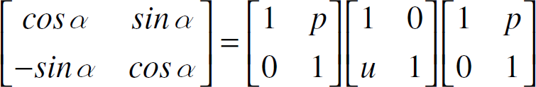
where p = (cosα − 1)/sinα and u = sinα. The angular increment α is chosen such that multiplication by p reduces to a bit shift. In stage 2, u = 2p/(1 + p²) can also be implemented as a bit shift if p < < 1. This approximation produces an error of less than 1 exact magnitude increases with p. This is a tradeoff to avoid floating point multiplication for every point. Thus, consecutive points on a circle can be computed in three steps involving bit shifts dictated by p, u, and p respectively as in Fig. 8.

Figure 8

Three-stage pipelined generation of points on circles.

This implies a delay of two clock cycles (with one or two stages executing at each edge) to evaluate the next point on the same circle. At any instant, only one stage of the pipeline is (two register sets are) active. So we can interleave the computation for the two circles in Fig. 6 such that points on two circles reach the output alternately. The angle counter is decremented only on alternate clock cycles.

Voting requires finding the first cell to vote and an adjacent cell subsequently. It is sufficient to compare a data point with cell boundaries, since the step size ensures vote in the existing or the adjacent cell. The voting process exploits inherent correlation between consecutive votes climinating computationally expensive divisions for each point.

Initially we employ binary logarithmic search to determine in O[log(N_grid)] cycles (n clock edges for a 2ⁿ × 2ⁿ grid), the first cell to be voted in the grid for each circle. Each of the 8 points on the circle lying partially in the grid must pursue this search independently, since information about voting of a cell by a point cannot be used to conclude about the vote of any other point on the circle. Observe that for the circle falling completely and symmetrically in the grid, the voting cell can be mirrored similar to points. For either circle, points mirrored over diagonals vote to a grid cell, only if it is different from cells voted by points being mirrored.

The voting process is further optimized in ADCs by accounting for the movement along either coordinate axes separately. Each data point, mirrored or otherwise should fall in the grid range for voting an example output of voting scheme for 16-cell grid is shown in Fig. 6. The cell(s) with maximum votes are potential candidates for the intersection of the two circles. To improve the resolution, these need to be examined with smaller angle increment by mapping this (these) cell(s) to the grid.

The architecture has been implemented in Xilinx 2V250CS144 device of Virtex II family for clock of 50 MHz with modular hierarchy preserved and fast optimization effort. The power and area obtained for the Flash converter, Streamlined divider modules and Main GPS unit from Synopsys FPGA Compiler II have been listed in the table below:

Module	Power (mW)	Area

Main GPS	1565	39449
Streamlined Divider	68.8	141
Flash Converter	391.89	1295

VI. Conclusions

Rigorous geometric analyses of visual landmark based terrain navigation have been presented. The new insights introduced in this paper may be summarized as:

an image of two landmarks helps to constrain the unknown geoposition of the aerial observer onto the surface of a unique toroid;

an image of three colinear landmarks reduces the same onto a uniquely defined circle, which is also perpendicular to the axis passing through the landmarks; and

the geoposition of an unknown ground location can be determined from a minimum of two image frames with three landmarks when the camera positions are known or already computed by using previous results.

We have also presented a Hough transform-like approach, facilitated by a class of CORDIC-structured computations based on the results of our analyses, that provides a fast and robust technique for compensating the GPS errors in locating the position of an aerial camera system, and a simple but effective solution to find positions of ground locations from images of them and known landmarks when INS is not available. The design integrates them with flash ADCs and forward plane rotation and has been implemented successfully to yield Cartesian coordinates of the observer. With N × N-cell voting grid, the resolution of coordinates improves at each iteration approximately by a factor of N. System has N_cordic + N_divider one-time computations and log(N_grid) − 2(π/ (4step)) iteration steps depending on resolution desired.

Footnotes

VII.

The author GS likes to acknowledge Harold Szu of Navy Surface Warfare Center for introducing this problem, and Scott Norton of Defense Technology Inc., for various insightful discussions. A portion of this work was supported by the National Science Foundation, through NSF-9612769; and, both the authors were with the Center for Advanced Computer Studies when this work was completed. The first author is now with the Air Force Institute of Technology; the scientific results contained in this report are those of the authors and do not necessarily represent the position of the U.S. Air Force or the Department of Defense.

References

Chatterji

Menon

, and Sridhar

, “GPS/Machine vision navigation system for aircraft,” IEEE Trans. Aerosp. Electron. Syst., 33, 3, 1012–1025, Jul., 1989.

Sridhar

and Pathak

, “Analysis of image-based navigation system for rotocraft low-altitude flight,” IEEE Trans. Syst., Man, Cybern., 22, 2, 290–299, Mar./Apr., 1992.

Rives

Bouthemy

Prasada

, and Dubois

, “Recovering the orientation and the position of a rigid body in space from a single view,” INRS-Telecommunications, 3, place du Commerce, Ile-des-Soeurs, Verdun, Quebec, Canada, Tech. Rep., 1981.

Fischler

and Bolles

, “Random sample consensus: A paradigm for model fitting with applications to image analysis and automated cartography,” Communications of the ACM, 24, 6, 381–395, Jun., 1981.

Horaud

Conio

Leboulleux

, and Lacolle

, “An analytic solution for the perspective 4-point problem,” Computer Vision and Pattern Recognition, Proceedings CVPR'89., IEEE Computer Society 1989.

Lowe

, “Three-Dimensional object recognition from single two-dimensional images,” Artificial Intelligence, 31, 355–395, 1987.

and Seetharaman

, “A Hough transform method for video assisted GPS in visual terrain navigation,” in Processings of the Third Indian Conference on Computer Vision Graphics and Image Processing. Ahmedabad, India., Dec., 2002.

USAF Scientific Advisory Board , “Unmanned aerial vehicles in perspective: Effects, capabilities and technologies. SAB-TR-03-01,” http://www.ae.utexas.edu/ASE261KChaput/reference-matl/UAVVol0Final.pdf, Tech. Rep., July, 2003.

Ahmed

Delosme

, and Morf

, “Highly concurrent computing structures for matrix arithmetic and signal processing,” Computer, 15, 1, 65–82, Jan., 1982.

10.

Illingworth

and Kittler

, “The adaptive Hough transform,” IEEE Trans. Pattern Anal. Machine Intell., 9, 5, 690–698, Sep., 1987.

11.

Roach

J. W.

and Aggarwal

J. K.

, “Determining the movement of objects from a sequence of images,” IEEE Trans. Pattern Anal. Machine Intell., 2, 6, 554–562, Nov., 1980.

12.

“The growing reach of unmanned vehicles,”

Springfield c4ISR - The Journal of Net-Centric Warfare, 4, 3, 2005.

13.

Faugeras

, Three-dimensional computer vision: A geometric view-point. Cambridge: MIT Press, 1993.

14.

Gellert

Gottwald

Hellwich

Kastner

, and Kustner

, The VNR concise Encyclopedia of Mathematics, 2nd ed. NY: Van Nostrand Reinhold, 1989.

15.

Hough

, “Method and Means for Recognizing Complex Patterns,” U.S. Patent 3069654, 1962.

16.

Ballard

, “Generalizing the Hough transform to detect arbitrary shapes,” Pattern Recognition, 13, 2, 111–122, 1981.

17.

Hill

F. S.

, “The pleasures of ‘Perp Dot’ products,” in Graphics Gems IV, Heckbert

P. S.

, Ed. San Diego: Academic Press, 1994, 138–148.

18.

Utgikar

Seetharaman

, and Le

, “A FPGA implementable architecture for video assisted GPS,” in Proceedings of the IEEE International Conference on Field Programmable Technology, 2003.

19.

Andraka

, “A survey of CORDIC algorithms for FPGA-based computers,” in Proceedings of the 1998 ACM/SIGDA Sixth International Symposium on FPGAs, 1998.

Video-Assisted Global Positioning in Terrain Navigation with Known Landmarks

Abstract

Keywords

I. Introduction

II. Imaging Model

Lemma 1

A. Geometric Analysis

Theorem 1

C. Special Configurations

Theorem 2

Theorem 3

Lemma 2

A. System Architecture

Footnotes

VII.

References