Sage Journals: Discover world-class research

Abstract

Some have suggested a threshold mechanism for the carcinogenicity of exposure to hexavalent chromium, Cr(VI). We evaluated the nature of the exposure—response relationship between occupational exposure to Cr(VI) and respiratory cancer based on results of two recently published epidemiological cohort studies. The combined cohort comprised a total of 2,849 workers employed at two U.S. chromate production plants between 1940 and 1974. Standardized mortality ratios (SMRs) for lung cancer in relation to cumulative Cr(VI) exposure categories were reported using regional mortality rates. Linear additive and multiplicative relative risk regression models were fit to the SMRs of the individual and combined studies. Both models fit the data from the individual studies reasonably well; however, the fit was somewhat less adequate for the pooled data. Meta-analysis of the slope estimates obtained from the multiplicative relative risk model showed substantial heterogeneity between the two epidemiological studies. In conclusion, these data indicate that a linear dose response describes the relationship between Cr(VI) and lung cancer reasonably well, and therefore these analyses do not necessarily support the threshold hypothesis for the lung carcinogenicity of Cr(VI). However, these results must be interpreted with recognition of the limitations of the use of epidemiological data in the evaluation of nonlinear exposure—response patterns.

Keywords

hexavalent chromium lung cancer exposure—response pattern meta-analysis

INTRODUCTION

The carcinogenicity of hexavalent chromium, CR(VI), has been well established, and the lungs are considered to be the primary target (IARC, 1990). Though hexavalent chromium readily transits cell membranes, several airway defense mechanisms exist, resulting in reduction to Cr(III) and/or elimination of Cr(VI) particles before reaching alveoli (De Flora, 2000). The human body's capacity to reduce and detoxify hexavalent chromium suggests a threshold mechanism. Indeed, some have suggested that Cr(VI) is carcinogenic only when the dose overwhelms the body's reduction capacity (Hathaway, 1989; De Flora, 2000). Resolution of this issue has important regulatory implications, especially with respect to exposure limits and environmental cleanup standards.

Although mechanistic and toxicological studies could be considered to provide the best evidence for a threshold mechanism (Hathaway, 1989), epidemiological studies may provide additional support for nonlinearity in the exposure—response relationship. We evaluated the evidence for nonlinearity of Cr(VI) carcinogenicity based on the results of two recently published epidemiological studies of chromate production workers (Gibb et al., 2000; Luippold et al., 2003).

METHODS

Study Population

The results of two recently published occupational cohort studies were considered in the evaluation of the nature of the exposure—response association between lung cancer and exposure to Cr(VI). One study included 482 workers employed at a Painesville, Ohio chromate production plant between 1940 and 1972 (Luippold et al., 2003). The second study comprised 2,357 workers employed at a Baltimore, Maryland, chromate production facility between 1950 and 1974 (Gibb et al., 2000). The vital status of workers in these cohorts was determined through 1997 and 1992, respectively. The total number of person-years was reported to be 14,048 (average duration of follow-up = 28.6 years) in the Painesville cohort and 70,736 (average duration of follow-up = 30.0 years) in the Baltimore cohort. The total number of lung cancer deaths was 51 and 122 in the Painesville and the Baltimore facilities, respectively.

Evaluation of Nonlinearity

Additive Relative Risk

To evaluate nonlinearity in the exposure—response data, we assumed that the number of lung cancer deaths follows a Poisson distribution. Subsequently, a linear nonthreshold multiplicative model was fit to categorical standardized mortality ratio (SMR) results using iteratively reweighted least-squares estimation with the procedure PROC NLIN in the SAS statistical software package (SAS Institute, Cary, NC; Hanley and Liddell, 1985; Hertz-Picciotto and Smith, 1993):

E [o b s_{i}] = α * E X P_{i} * (1 + β * x_{i})

where E[ ] indicates the expectation of a random variable, obs_i is the observed number of deaths at exposure level i, α represents any difference between the study cohort and the external referent population with respect to baseline rate, EXP_i is the expected number of deaths at exposure level i, β represents the increase in the relative risk per unit of exposure, and x_i is the exposure level in mg/m³-years.

The standard error to the slope was also estimated. A goodness-of-fit chi-square statistic based on a comparison of theoretical prediction vs. empirical observation,

χ^{2} = \sum_{i} \frac{{(o b s_{i} - p r e d_{i})}^{2}}{p r e d_{i}}

was computed to determine the fit of the model, in addition to visual inspection of the plotted model and data points.

Multiplicative Relative Risk

As an alternative to the additive relative risk model, slope estimates were obtained by fitting a linear trend model to the natural logarithm of the SMRs (i.e., ln(SMR)) reported across exposure levels. For the calculation of the slope, we assume that ln(SMR) follows a normal distribution. Linear models were fit to the study results using weighted least-squares estimation with the procedure PROC REG in SAS:

S M R_{i} = e^{β * x_{i}}

where SMR_i is the relative risk at exposure level i, β represents the increase in natural logarithm of the relative risk per unit of exposure, and x_i is the exposure level in mg/m³-years.

The weights were determined by the inverse of the variance of ln(SMR) (Greenland, 1987):

var [ln (S M R_{i})] = {[\frac{ln (U C L_{i}) - ln (L C L_{i})}{3.92}]}^{2}

where UCL and LCL are the 95% upper and lower confidence limits of the SMR, respectively. The standard error of the slope estimate was also calculated. Visual inspection of the plotted model and data points, and the goodness-of-fit chi-square statistic, were used to determine the fit of the model.

Pooled Analysis

First, linear regression models were applied to the categorical risk estimates presented in the individual studies. For the exposure—response analysis of the Painesville data, we employed the midpoint of each exposure category except for the highest group, for which we added one-half the width of the previous interval. Gibb and colleagues reported the mean exposure level for each cumulative exposure category. In addition, slope estimates were derived based on the pooled exposure—response data, which included nine exposure categories. In both studies, SMRs for lung cancer in relation to cumulative Cr(VI) exposure were computed using regional mortality rates, adjusting for gender, race, and calendar year. Furthermore, both studies employed a 5-year lag, thereby enabling us to pool the data to evaluate the exposure—response relationship over a wide range of exposure levels.

Meta-Analysis

Pooling of the exposure—response data may be inappropriate due to differences in the characteristics of the workforces in the two epidemiological studies (Luippoldet al., 2003). Therefore, a random effects model was applied to the slope estimates obtained with the multiplicative relative risk model to evaluate any heterogeneity between the two studies, using PROC MIXED in SAS (Tweedie and Mengersen, 1995; Normand, 1999; Sheu and Suzuki, 2001).

RESULTS

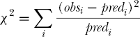
The findings of the two epidemiological studies are presented in Table 1 and in Figures 1 and 2. The exposure—response association reported for the Baltimore cohort appeared to be slightly supralinear, whereas the relationship presented for the Painesville cohort was approximately linear despite some inconsistencies in the lower exposure categories.

FIGURE 1

Standardized mortality ratios (SMRs) and 95% confidence intervals in relation to cumulative exposure to Cr(VI) reported by Gibb and colleagues (Gibb et al., 2000) and predicted relative risks (solid line = additive relative risk model; broken line = multiplicative relative risk model).

FIGURE 2

Standardized mortality ratios (SMRs) and 95% confidence intervals in relation to cumulative exposure to Cr(VI) reported by Luippold and colleagues (Luippold et al., 2003) and predicted relative risks (solid line = additive relative risk model; broken line = multiplicative relative risk model).

TABLE 1

Cumulative Exposure to Hexavalent Chromium in Relation to Lung Cancer Mortality in Two Occupational Cohorts of Chromate Workers, 5-year lag

Mean (mg/m³-years)*	Obs	Exp	SMR	95% CI
Gibb et al.
0.00023	26	27.1	0.96	0.63–1.38
0.0022	28	19.1	1.42	0.95–2.01
0.016	30	19.1	1.57	1.07–2.20
0.23	38	17.0	2.24	1.60–3.03
Luippold et al.
0.10	3	4.5	0.67	0.14–1.96
0.35	8	4.4	1.84	0.79–3.62
0.77	4	4.4	0.91	0.25–2.34
1.88	16	4.4	3.65	2.08–5.92
3.53	20	4.3	4.63	2.83–7.16

Units of CrO₃/m³-years reported by Gibb et al. converted to units of Cr(VI)/m³-years (ratio of molecular weights = 1.92); midpoint for Luippold et al.

Table 2 shows the slope estimates and the fit statistics for both relative risk models applied to the findings of the individual studies. The slope estimate obtained from the additive relative risk model was about two-fold higher for the Gibb study compared to the Luippold study. This difference was even greater when the multiplicative relative risk model was applied. Nevertheless, the fit of the models was generally satisfactory with the exception of the fit of the multiplicative relative risk model to the Gibb findings. Similar conclusions were reached based on visual inspection of the slopes (Figures 1 and 2).

TABLE 2

Slope Estimates and Goodness-of-Fit Statistics for Linear Regression Models

Study	Additive relative risk†		Multiplicative relative risk†

	Slope (SE)	Goodness-of-fit p-value	Slope (SE)	Goodness-of-fit p-value
Individual studies
Gibb	3.53 (2.08)	0.18	3.61 (1.14)	0.03
Luippold	1.58 (1.15)	0.26	0.48 (0.07)	0.20
Pooled data	0.75 (0.31)	0.06	0.50 (0.12)	0.00004

†

See text for explanation; SE = standard error.

The fit of the models to the pooled data was generally inadequate based on both model fit statistics (Table 2) and visual inspection (Figure 3), predominantly due to a poor fit at low levels of exposure. Furthermore, the meta-analysis of slope estimates obtained from the multiplicative relative risk model showed a substantial amount of heterogeneity between the two studies (p-value for heterogeneity = 0.006; data not shown), indicating that pooling the findings of the two studies may not be appropriate.

FIGURE 3

Standardized mortality ratios (SMRs) and 95% confidence intervals in relation to cumulative exposure to Cr(VI) based on pooled results, and predicted relative risks (solid line = additive relative risk model; broken line = multiplicative relative risk model).

DISCUSSION

The analyses presented here indicate that data from the two most informative epidemiological studies available to date, considered either separately or combined, do not support the threshold hypothesis for the lung carcinogenicity of Cr(VI). However, the limitations of the use of epidemiological data in the evaluation of nonlinear exposure—response patterns must be acknowledged (Smith and Sharp, 1985; Smith, 1988; Hathaway, 1989; Hertz-Picciotto, 1995; Stayner et al., 1999).

First, in epidemiology there are usually insufficient data points to reject linearity (Wright et al., 1997). Furthermore, epidemiological data are subject to several biases that may mask or produce nonlinear exposure—response associations, including exposure misclassification, confounding by smoking, confounding by other occupational carcinogens, the healthy worker survivor effect, and other biases (Hertz-Picciotto and Smith, 1993; Mundt and May, 2001; Stayner et al., 2003). Although it is unlikely that confounding by smoking could drive the observed exposure—response patterns (Gibb et al., 2000; Luippold et al., 2003), the impact of other biases is more difficult to determine. Bias due to exposure misclassification is likely to be one of the strongest determinants of finding or failing to find a particular dose-response relationship in epidemiological data.

The analyses presented here have several additional limitations. First, it should be noted that comparisons of SMRs between categories of exposure are strictly invalid if their confounder distributions differ (Checkoway et al., 1989); however, the extent of any bias is generally believed to be small (Breslow et al., 1983; Greenland, 1998). In addition, the difference in study populations hampers the comparability of the results of the two studies (Luippold et al., 2003). Painesville workers with less than one year of employment were excluded from further study, whereas a large proportion of the Baltimore cohort included workers employed for less than one year. Consequently, workers in the Baltimore cohort may have different risk profiles than Painesville workers (e.g., due to differences in lifestyle factors). Indeed, the meta-analysis indicates that there is substantial heterogeneity between the two cohorts in lung cancer risk due to occupational Cr(VI) exposure and that pooling their results may not be appropriate.

It is possible that the data from the Painesville study reflect a threshold effect, because visual inspection of the data suggests very weak or no elevation in risk at cumulative exposure levels less than 1.9 mg/m³-years and clearly elevated SMRs for exposures equal to or exceeding 1.9 mg/m³-years (Figure 2). However, interpretation of the presented data is hampered by arbitrary categorization of cumulative exposure and assumptions about the midpoints of these exposure categories, which may have resulted in an inaccurate representation of the true exposure-response association. Further insight into the presence or absence of a threshold effect may be gained from analysis of the original study data using spline regression models (Greenland, 1995; Boucher et al., 1998).

References

Boucher

Slattery

Berry

Quesenberry

Anderson

. Statistical methods in epidemiology: A comparison of statistical methods to analyze dose-response and trend analysis in epidemiologic studies. J Clin Epidemiol. 1998; 51: 1223–1233.

Breslow

Lubin

Marek

Langholz

. Multiplicative models and cohort analysis. J Am Stat Assoc. 1983; 78: 1–12.

Checkoway

Pearce

Dement

. Design and conduct of occupational epidemiology studies: II. Analysis of cohort data. Am J Ind Med. 1989; 15: 375–394.

De Flora

. Threshold mechanisms and site specificity in chromium(VI) carcinogenesis. Carcinogenesis. 2000; 21: 533–541.

Gibb

Lees

Pinsky

Rooney

. Lung cancer among workers in chromium chemical production. Am J Ind Med. 2000; 38: 115–126.

Greenland

. Quantitative methods in the review of epidemiologic literature. Epidemiol Rev. 1987; 9: 1–30.

Greenland

. Dose-response and trend analysis in epidemiology: Alternatives to categorical analysis. Epidemiology. 1995; 6: 356–365.

Greenland

. Meta-analysis. In: Greenland

, ed. Modern Epidemiology. Philadelphia, PA: Lippincott-Raven; 1998: 643–673.

Hanley

Liddell

. Fitting relationships between exposure and standardized mortality ratios. J Occup Med. 1985; 27: 555–560.

10.

Hathaway

. Role of epidemiologic studies in evaluating the carcinogenicity of chromium compounds. Sci Total Environ. 1989; 86: 169–179.

11.

Hertz-Picciotto

. Epidemiology and quantitative risk assessment: A bridge from science to policy. Am J Public Health. 1995; 85: 484–491.

12.

Hertz-Picciotto

Smith

. Observations on the dose-response curve for arsenic exposure and lung cancer. Scand J Work Environ Health. 1993; 19: 217–226.

13.

International Agency for Research on Cancer (IARC). Chromium, Nickel and Welding. Lyon, France: IARC; 1990.

14.

Luippold

Mundt

Austin

Liebig

Panko

Crump

Proctor

. Lung cancer mortality among chromate production workers. Occup Environ Med. 2003; 60: 451–457.

15.

Mundt

May

. Epidemiological assessment of hormesis in studies with low-level exposure. Human and Ecological Risk Assessment. 2001; 7: 795–809.

16.

Normand

. Meta-analysis: Formulating, evaluating, combining, and reporting. Stat Med. 1999; 18: 321–359.

17.

Sheu

Suzuki

. Meta-analysis using linear mixed models. Behav Res Methods Instrum Comput. 2001; 33: 102–107.

18.

Smith

. Epidemiologic input to environmental risk assessment. Arch Environ Health. 1988; 43: 124–129.

19.

Smith

Sharp

. A standardized benchmark approach to the use of cancer epidemiology data for risk assessment. Toxicol Ind Health. 1985; 1: 205–212.

20.

Stayner

Bailer

Smith

Gilbert

Rice

Kuempel

. Sources of uncertainty in dose-response modeling of epidemiological data for cancer risk assessment. Ann NY Acad Sci. 1999; 895: 212–222.

21.

Stayner

Steenland

Dosemeci

Hertz-Picciotto

. Attenuation of exposure-response curves in occupational cohort studies at high exposure levels. Scand J Work Environ Health. 2003; 29: 317–324.

22.

Tweedie

Mengersen

. Meta-analytic approaches to dose-response relationships, with application in studies of lung cancer and exposure to environmental tobacco smoke. Stat Med. 1995; 14: 545–569.

23.

Wright

Lopipero

Smith

. Meta-analysis and risk assessment. In: Savitz

, ed. Topics in Environmental Epidemiology. New York: Oxford University Press; 1997: 28–63.

Evaluation of the Exposure—Response Relationship of Lung Cancer Mortality and Occupational Exposure to Hexavalent Chromium Based on Published Epidemiological Data

Abstract

Keywords

INTRODUCTION

METHODS

Study Population

Evaluation of Nonlinearity

Additive Relative Risk

Multiplicative Relative Risk

Pooled Analysis

Meta-Analysis

RESULTS

DISCUSSION

References