
Abstract
In the context of the French 500-m deep radioactive waste repository, electrochemical impedance spectroscopy and a methodology based on complex impedance analysis were carried out to follow the hydration of grout containing cement–bentonite mixture and iron corrosion together. The grout was initially a paste, and solidified with time. After a 100-day-curing, the temperature of the system (grout + steel) was increased from room temperature to 80°C to simulate the effect of a nuclear waste overpack. At room temperature, the ionic conductance exhibited a continuous decrease followed by an increase at 80°C. After an initial drop, the corrosion rate increased to a quasi-steady state value at around 1.5 µm/year at 21°C. At 80°C, the corrosion rate increased to about 30 µm/year before gradually dropping to much lower values. Eventually, then the passivation of iron seemed to occur since the corrosion rate has decreased continuously down to 0.1 µm/year.
This paper is part of a supplement on the 6th International Workshop on Long-Term Prediction of Corrosion Damage in Nuclear Waste Systems.
Introduction
In the context of the French radioactive waste repository, Andra has developed a 500-m deep disposal concept for the high-level waste (HLW). It plans to inject a grout containing cement–bentonite mixture between the steel liner and the wall of a HLW cell drilled in the Callovo-Oxfodian layer [1]. This mixture (or grout) has two main functions. The first one is to neutralise any acidity due to the oxidation of the sulphur-containing species in the claystone after drilling operation. For example, the oxidation of pyrite can be described as follows:

The second one is to limit the oxygen diffusion into the claystone during the exploitation phase. The pH in the genuine claystone at room temperature is about 7. The unaltered cement in the environment implies that the pH in the vicinity of the liner will be alkaline (10 < pH < 13). Over time, the pH should decrease to return to that of Callovo-Oxfordian clay because of leaching of the cement phases. Since the canisters are a source of heat, the pH is likely 6 at 90°C. During the first few years, the basic pH of the grout should allow passivation of the steel. This passivation should be preserved at long times even if there is acidification of the steel environment. Indeed, other works showed that iron passivated at pH = 6 at 90°C even if this passivation did not occur until several months [2]. In this scenario, the corrosion rate of steel should always remain moderate even if a transient increase is expected due to the acidification of the environment. In that study, the corrosion rate of Armco® iron (the same used in this study) decreased to 0.3 μm/year after 2 years of testing [2].
For this preliminary experiment, we used a tentative composition of a bento-cementitious mixture. No effort was put on its chemical characterisation. From a qualitative point of view, it is possible to say that the pH was around 12.3 when the mixture was put in place. It is the equilibrium pH of portlandite usually detected at the young age. Indeed, this mixture at the early stage should have behaved like a low pH cement, from which its formula is based. This transitory pH should have evolved when portlandite disappeared and calcium silicate hydrate controlled the chemistry of the mixture. To our knowledge, pH should have then stabilised around 11 (at 25°C, i.e. around 10-10.5 at 80°C) until the end of the experiment. The next experiment will aim to have a better understanding of the evolution of a new clay–cement mixture.
Electrochemical impedance spectroscopy (EIS) was carried out to follow (i) the hydration of cementitious oxides in the grout and (ii) the iron corrosion, both at room temperature and at 80°C, to simulate the introduction of nuclear waste canisters in the liner. A methodology based on complex impedance analysis was developed to extract the different parameters at high and low frequencies of the spectra.
Experimental set-up
For this preliminary experiment, the grout was made of 16% CEM III/C Rombas, 4% Bentonite and 80% Evian® mineral water. The experiment was performed in autoclave at 21°C in initial aerated condition for 100 days to simulate sealing. Subsequently, the temperature was increased at 80°C to simulate the effect of a nuclear waste package emplaced in contact with it. So both the corrosion of iron and the curing of the cement–bentonite mixture occurred in fully closed condition.
The autoclave body consisted of AISI 316L stainless steel, which also served as the counter electrode. A picture of the autoclave head is shown in Figure 1. It is possible to distinguish at the back, the glove finger which receives the thermocouple used for measuring the temperature in the autoclave, which was recorded by an Agilent acquisition apparatus. In the foreground, there are three electrodes. One electrode was arbitrarily chosen as pseudo-reference and another one as working electrode. The two lateral passages accommodate the Armco® iron electrodes of 47.1 cm2. Armco® iron is a pure (99.85%) ferritic iron with low carbon (C < 0.02%). The electrodes were polished with Si–C (Struers) polishing sheets up to grade 4000. In the centre is the third electrode. Its surface is 15.7 cm2 and is made of nickel coated with 200-300 nm of gold obtained by physical vapour deposition. This gold electrode was used to study the redox activity of the grout. But the results obtained were suspicious, since grout–gold interaction has occurred. In particular, they were indicative that the gold electrode was ‘inhibited’, since no decrease of its impedance occurred after the temperature was increased. The electrical insulation of the electrodes is ensured by tubes of zirconium oxide stabilised with yttrium. These tubes were supplied by DEGUSSIT® (reference FZY) and machined by the company UMICORE®.
Picture of the experimental set-up.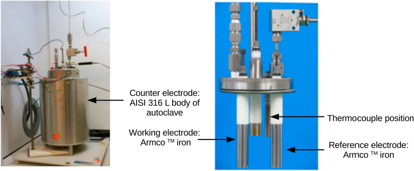
The cement paste was simply poured into the autoclave and the electrodes were immersed in it.
EIS was performed at open circuit potential in the 100 kHz to 0.1 mHz frequency range using a 10 mV sine-wave amplitude with a Biologic SP-200 potentiostat. EIS gave two kinds of results. In the high frequency range (100-1 kHz), data linked to the ionic conductance of the mixture were acquired. In the low frequency range (1-0.1 mHz), the corrosion rate could be evaluated thanks to the Stern–Geary method [3].
Experimental results
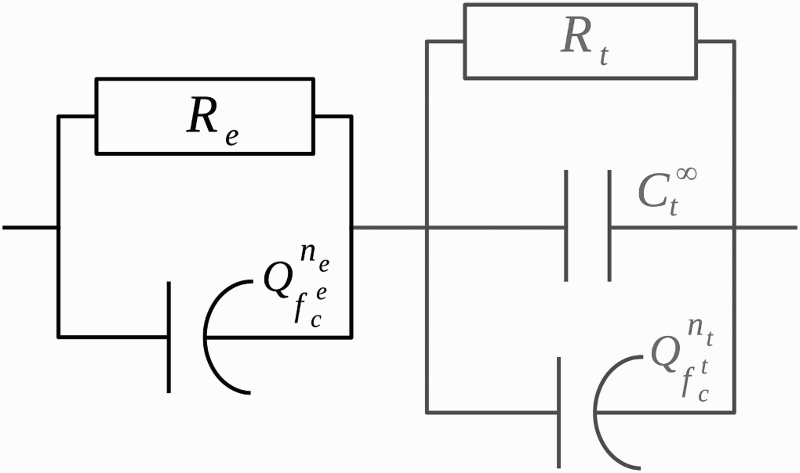
An example of Nyquist diagram of iron in cement–bentonite paste is shown in Figure 2. The insert corresponds to the high frequency range. A loop related to the grout at high frequency and another related to the iron at lower frequencies are identified. Thus, the following equivalent circuit is proposed in Figure 3.
Nyquist diagram of iron in cement–bentonite mixture at 4 days at 80°C after 107 days at 21°C, so a total of 111 days (high frequency data used to determine the cement impedance are described by black crosses, low frequency data, used to calculate the corrosion rate of iron, are presented with grey circle). Insert: zoom of the high frequency part. Equivalent circuit of the system.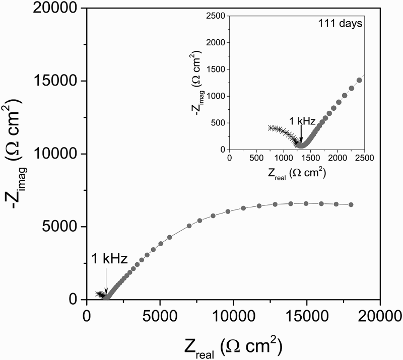
Evaluation of the ionic resistance
Methodology
In simple systems in the Nyquist representation, the intercept of the curve with the real axis at high frequency gives an estimate value of the electrolytic resistance Re (Ohm) since the impedance of capacitive components ( ) goes to zero.
In our system, the evidence of a loop at high frequency makes the determination of Re a little bit tricky. To analyse such capacitive loop (insert in Figure 2), it is convenient to use the complex capacitance which is defined by [4,5]:
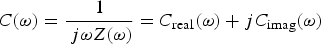
The complex capacitance representation is well adapted for analysing parallel contributions since the whole contribution is the sum of each contribution.
In the present study, the high frequency loop represented in dark in Figure 2 could be simulated by an equivalent circuit with a resistance (Re) in parallel with a constant phase element (Qe), as shown in Figure 3:
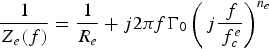
 is the characteristic frequency (in Hz) of the Qe. ne is an exponent with −1 < ne ≤ 0. Γ0 = 1 F cm−2 for unit consistency, which avoids getting a Qe constant unit depending on the exponent ne, as usually done in the literature.
The resistance Re corresponds to the response of the continuous ion-conducting paths. The contribution of the ionic conductor discontinuous paths corresponds to the Qe [6]. These discontinuous paths do not allow the transport of ions over large scales, i.e. the transport is confined within ended segments. In these segments, there is accumulation of positive or negative charges at the ends of the paths during one half wave sine and opposite charge accumulation during the next alternation. This accumulation of charges corresponds to a capacitance-like impedance. For a fixed frequency, the lower the segment length, the higher the charge accumulation if the wave reaches the pore ends.
The expression of the complex capacitance Ce(f) derived from (3) is
Representation of the (a) log 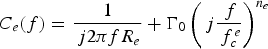
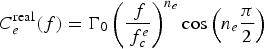
 vs. log f in order to determine the values of
  and ne as shown in Figure 4(a):

 (circle), log
  (square) and (b) log
  and log
  (triangle) as a function of log of the frequency for the high frequency data used described by black crosses in Figure 2. The lines represent the linear fitting used to estimate the values of
  and ne (on (a)) and Re (on (b)).
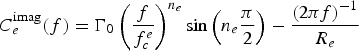
Finally, plotting (8) in log–log scale (Figure 4(b)), the value of Re could be determined by linear fitting and validation of the correction was ensured by the evidence of a slope equal to −1. In this example, the correction was necessary only for frequency higher than 10 kHz.
Results
In Figure 5(b), the decrease with time of the position of the straight line indicates an increase in the value of Re. This increase corresponds to a decrease of the admittance Ye which is directly proportional to the ionic DC conductivity. The proportional coefficient was unknown since the cell geometry was not simple (planar or cylindrical). But, it was constant. Initially, the cement–bentonite mixture was a paste, i.e. solid particles were embedded in mineral water. With time, this mixture solidified. This process corresponds to the built-in of a solid phase containing pores filled with ionic solution. As a consequence, the seeming ionic conductance of the mixture has decreased with time.
Evolution of (a) log  and (b) log
  as a function of frequency from 21 to 100 days at 21°C.
From the 107th day, to simulate the effect of the hot nuclear waste, the temperature of the system was increased up to 80°C. At this temperature, an inverse trend was observed as displayed on the curves in Figure 6(b). The ionic DC conductivity of the grout continuously increased with time. The same trends have been obtained for the frequency variation of log Evolution of (a) log  (see Figures 5(a) and 6(a)). For the moment, such variations cannot be interpreted. They are likely due to the evolution of occluded pores. But to go further, modelling of the pore structure would be needed. This was out of the scope of this paper. This paper shows, however, that EIS could be used to monitor qualitatively geochemical evolution of the grout. But EIS cannot identify the geochemical evolution.
 and (b) log
  as a function of frequency between 111 and 162 days at 80°C.
As shown in Figure 7, at 21°C the DC ionic conductance Ye has decreased continuously. From this time evolution, it could be concluded that the curing time of the mixture was about 100 days at 21°C. It must be emphasised that in the range 80-100 days, some slow decrease for Ye could still be observed. But this decrease was lower and lower with increasing time.
Time evolution of the ionic conductance Ye of the cement–bentonite mixture.
At 80°C, an increase was observed. But this increase was delayed. This was evident that the changes are not directly related to the effect of temperature on ionic admittance but rather to geochemical transformations. Such the geochemical transformations were not instantaneous with the increase of the temperature. This delay was expected since geochemical transformation needs time to proceed (kinetic processes). Then EIS could give qualitative information about the kinetics of the transformations.
Corrosion monitoring of iron
Methodology
The evaluation of the corrosion rate is obtained with the low frequency part of the impedance spectrum (represented in grey circles in Figure 2). As described below, a methodology based on complex capacitance was used [4,5]. As shown in [5], the use of complex capacitance spectrum is relevant only if an accurate correction of serial ionic Re was done. In the present study, the ionic contribution is not reduced to a pure resistance as shown previously. But the processing would be the same if the complex impedance Ze is subtracted in place of Re.
The expression of the complex capacitance Ct(f) derived from Zt(f) is
It is important to notice that the Ze(f)  ℂ as Z exp(f), so in the middle frequency range, Ze(f) and Z exp(f) overlap even if Ze(f) is not the major contribution.
The ion conduction process of the cement–bentonite mixture characterised by Ze and the corrosion process characterised by Rt take place in series since the current through the corrosion interface must then be transported by the environment.
The subtraction Z exp(f)–Ze(f) allowed the determination of the iron-grout impedance Zt(f). Then, it was assumed that the equivalent circuit for Zt(f) was a resistance Rt in parallel with CPE, Qt, with a capacitance  in parallel (see Figure 3). So the complex capacitance Ct(f) is

 in F cm−2,
  is the characteristic frequency in Hz and nt
  ]−1,0[.
The Q Jonscher complex capacitance was analysed at high frequency range of Zt(f) or Ct(f), where the term  is small compared with the two others terms in (10), which corresponds to a Jonscher's relation [7,8].
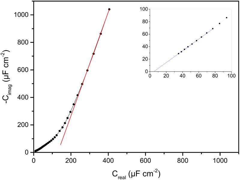
The capacitance was estimated as the intercept of the imaginary part as the function of the real part of the complex capacitance in the Cole–Cole representation [9,10] which is similar to the Nyquist representation for impedance, as shown in Figure 8. In other words, the estimation of Cole–Cole representation of iron in cement–bentonite mixture at 4 days at 80°C after 107 days at 21°C, so a total of 111 days. for capacitance spectrum is the mirror image of the estimation of Re for impedance spectrum:
 and nt in the low frequency range (as (7)). Then the charge transfer resistance Rt was determined in the same way than those used to determine Re in the previous section.
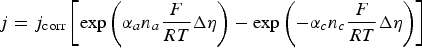
The evaluation of the iron corrosion rate has been performed thanks to the Stern–Geary method. At free corrosion potential, j corr, is equal to the anodic or to the opposite of the cathodic current densities given by Butler–Volmer laws [11]:

It is important to note that αi is inversely proportional to the Tafel plots coefficient βi currently used in the literature [12].
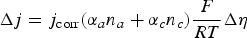
In the vicinity of the free corrosion potential, the Faradic current density is given by
If Δη is small enough, the exponentials could be replaced by their Taylor series restricted to the first order [12]:
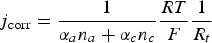
 ). The number of electrons involved in the cathodic process is generally nc = 1 because the reduction processes of oxidant in solution involve several steps of single electronic exchange and in most cases only one is the limiting step. Currently, the Butler–Volmer coefficient is assumed to be around 0.5. So αcnc ≈ 0.5. na is equal to the oxidation degree of iron which could be 2 or 3. The evaluation of αa is more tricky since it depends on oxidation model considered. In the framework of the Tafel approach, αa is linked to the slope of the anodic current–voltage curve. In the passive iron case, the anodic current–voltage curve is flat. So, αa ≈ 0 and so αana ≈ 0. On the contrary, in the framework of the point defect model, Macdonald and co-workers [13] have shown that αa ≈ 0.5 and na = 3. Then αana ≈ 1.5. In summary, in the framework of the Tafel approach, αana + αcnc ≈ 0.5, whereas in the framework of the PDM, αana + αcnc ≈ 2.
This implies that for a same value of Rt, the corrosion current density is four times higher for the Tafel approach than for the PDM approach. To be conservative, the higher value of was used and taken to 2.
From the current density of corrosion j corr in A cm−2, the corrosion rate in µm/year is calculated by the Faraday law:
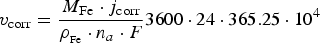
The number of electrons involved in the oxidation of Fe is 2 or 3 (anodic process). It was chosen to take an average value, na = 2.5 ± 0.5 (relative error of 20% on the corrosion rate value) in order to consider both options.
Results
The time evolution of the charge transfer resistance (Rt) and the iron corrosion rate (ʋ corr) in the cement–bentonite mixture at 21 and 80°C are presented in Figure 9. During the curing period at 21°C, after an initial decrease during the first 5 days to ≈ 0.2 μm/year, the corrosion rate increased extending up to about 60 days to quasi-steady state value around 1.5 µm/year. This result was in contrast to those obtained for the monotonic time evolution of the ionic conductance shown in Figure 7. The decrease in corrosion rate observed in the first 5 days could be related to the setting of the cement–bentonite mixture, in particular to decrease of the available aerated water for iron corrosion. However, the following increase and the sudden decrease could not be explained because the curing process of the mixture would continuously decrease the amount of free water available for iron corrosion. This contradiction suggests that the corrosion rate does not depend on the amount of free water only. Two chemical features could be considered. One was the evolution of the pH of the free porewater. The second was the amount of dissolved oxygen available for iron corrosion. This oxygen has been likely consumed by the cathodic reduction on all the metal surfaces inside the autoclave and especially the body of the autoclave.
Time evolution of the charge transfer resistance (grey open square) and iron corrosion rate (black circle) in the cement–bentonite mixture.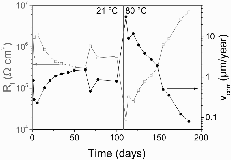
The increase of the temperature up to 80°C induced an increase of the corrosion rate by thermal activation to about 30 µm/year followed by a decrease to much lower levels. Then, the passivation of iron seemed to occur, since the corrosion rate decreased down to ≈ 0.1 µm/year. The protectiveness of the passive layer was first relatively low but was enhanced at longer time (at 80°C). Note that no correlation of the corrosion rate with changes in ionic conductance was observed across the whole experiments. This shows that the two loops are connected to different processes.
Figure 10 shows the damage curve versus time. It was obtained from the integration by the trapezoidal method of ʋ corr curve versus time (Figure 9). After 200 days, the damage was estimated at 1.5 μm. This value is consistent with the appearance of the electrode observed during the disassembly of the experiment since the initial polished surface state was preserved (Si–C grade 4000). Only a slight green halo was observed. As a consequence, no cross-sectional observations have been performed. It must be outlined that the corrosion monitoring has given only a coarse order of magnitude value of the iron corrosion rate, considering the assumptions used. Nevertheless, the trend towards passivation of iron was clearly evidenced.
Time evolution of the iron damage in the cement–bentonite mixture.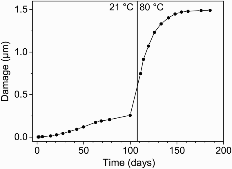
Conclusion
This study is a preliminary investigation. The results presented in this article evidenced that it was possible to perform in situ corrosion monitoring of iron in cement–bentonite mixture and to follow the hydration of the grout by EIS and complex capacitance analysis. No correlation between the corrosion and ionic conductance was observed across the whole experiment. At room temperature, the iron corrosion rate was about 1.5 µm/year. The temperature increase up to 80°C made the corrosion rate rise to around 30 µm/year before gradually dropping to much lower values. Eventually, then the passivation of iron seemed to occur at high temperature since the corrosion rate has decreased continuously down to 0.1 µm/year. The total damage was estimated at 1.5 µm.