Sage Journals: Discover world-class research

Abstract

The power law model produces both temperature varying and unreliable estimates for its parameters. Threshold stresses have been suggested as a solution. The power law and Wilshire models are modified to include this stress and estimation and error decomposition methods applied to assess its importance in representing failure times. A statistically significant and temperature-dependent threshold stress was identified in two low-alloy steels. This threshold stress was closer to the operating stress in the Wilshire model. The inclusion of this stress reduced interpolation errors, but this improvement was greater in the Wilshire model. The Wilshire model increased the random component of these errors at all temperatures in one material, but only at some temperatures for the other.

Keywords

Power law creep Wilshire equation threshold stress low-alloy ferritic steel

Introduction

Low-alloy ferritic steels such as 1Cr–0.5Mo, 1Cr–1Mo–0.25V, 2.25Cr–1Mo and 0.5Cr–1Mo–1V are extensively used for high temperature applications in the power generation and petro-chemical industries. This is because they all have good creep strength together with good resistance to oxidation and hydrogen embrittlement at the elevated temperatures required within these sectors. The main applications for these steels are in components such as turbine rotors and steam pipes/headers. Typically, the components used within the power generation sector operate at a temperature and stress of around 823 K and 50 MPa, respectively. 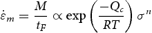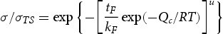The minimum creep rate, ${\dot{ε}}_{m}$ , and times to failure t_F for the above-mentioned materials have typically been described using variants of a power law relationship of the form

{\dot{ε}}_{m} = \frac{M}{t_{F}} \propto \exp (\frac{- Q_{c}}{R T}) σ^{n}

(1)

where Q_c is the activation energy for self diffusion in the bulk matrix, R is the universal gas constant, T is the absolute temperature and σ is the applied stress. M (the Monkman-Grant parameter) and n (the stress exponent) are model parameters requiring determination from the experimental data. Other parametric models strongly based on this power law model include those developed by Larson and Miller [1], Manson and Haferd [2], Manson and Brown [3], Manson and Muraldihan [4], Trunin et al. [5] and Orr et al. [6].

However, these power law-based approaches have several known weaknesses that are now well documented and include the derivation of unrealistic values for the activation energy and stress exponent (which also appears to vary with both stress and temperature) when these models are applied to creep data on materials used for high temperature applications. The development of the Wilshire equations [7] was driven by a desire to overcome this problem of an unrealistic and varying stress exponent. A fundamental feature of this new approach was the normalisation of the applied stress through use of the ultimate tensile strength. What was new about this stress normalisation was that the approach constrained failure times to zero when the test stress equalled the tensile strength and infinity when stress equalled zero. This was done using a ‘Weibull’ type expression of the form:

σ / σ_{T S} = \exp {- {[\frac{t_{F}}{k_{F}} \exp (- Q_{c} / R T)]}^{u}}

(2)

where Q_c is the activation energy for self diffusion in the bulk matrix, σ_TS is the tensile strength measured at temperature T and k_F and u are the unknown parameters of the model. Research efforts using this approach have concentrated on the application of the model to a wide variety of engineering alloys [8–11] and has been partially successful in stabilising the unknown parameters. The unknown parameters k_F and u for many materials appear more stable than in the power law model – remaining constant over wider stress and temperature ranges – changing only at one or two critical stress values (often around the yield stress) where a change in creep mechanism is identified. However, variation in this model's parameters still remains.

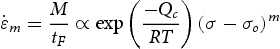
It has been suggested that observing unrealistic n values of more than 5 is the result of not accounting for threshold stress. Williams and Wilshire [12], for example, suggested that creep occurs not under the full applied stress, but under a reduced effective stress (σ − σ₀), so that the power law model is more correctly written as

{\dot{ε}}_{m} = \frac{M}{t_{F}} \propto \exp (\frac{- Q_{c}}{R T}) (σ - σ_{o})^{m}

(3)

where σ₀ can be regarded as either a friction stress by the proponents of dislocation climb [13,14], or as a back-stress by the proponents of dislocation glide models of creep [15]. σ₀ is also commonly referred to as a threshold stress. Such authors as those above have suggested that with an appropriate choice for σ₀, m can be made independent of test conditions with the activation energy then being equal to that for self-diffusion through the crystal lattice. They argued that the inclusion of σ₀ will result in m having a value between 5 and 7 for dislocation glide and a value between 3 and 5 for diffusion-controlled dislocation climb.

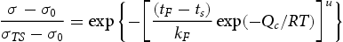
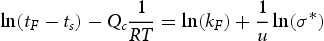
If it is the effective stress that is important, then the Wilshire equation should also be rewritten as

\frac{σ - σ_{0}}{σ_{T S} - σ_{0}} = \exp {- {[\frac{(t_{F} - t_{s})}{k_{F}} \exp (- Q_{c} / R T)]}^{u}}

(4)

In this reformulation, failure will occur either instantaneously (if t_F = t_s = 0), or in a very short period of time given by t_s, when σ = σ_TS. σ₀ is a threshold stress such that for specimen's placed on test under such a condition, the specimen will never fail. In this reformulation, t_F → t_s as σ → σ_TS, i.e. as

\frac{σ - σ_{0}}{σ_{L S} - σ_{0}} \to 1

. Further, t_F →

\infty

as σ → σ₀, i.e. as

\frac{σ - σ_{0}}{σ_{L S} - σ_{o}} \to 0

The presence of a threshold stress is not as well established for creep failure as it is for fatigue, but authors have tried to explain its existence in different ways depending on the material under investigation. For low-alloy ferritic steels, microstructural changes tend to develop after prolonged service at high temperature and this mainly consists of the coarsening of carbides, compositional and morphological changes in the carbides, and increases in the inter-particle spacing formation of new carbides. Research by Senior [16], Singh and Banerjee [17,18] and Cheruvu [19] have revealed that such microstructural changes only lead to a degradation in creep strength after long exposure at lower stress levels (and so by implication also at lower temperatures) – given the long exposure required for such coarsening. As a result of this, at low stresses (long-term rupture strengths) virgin and service exposed materials were hardly distinguishable, suggesting the presence of a threshold stress induced by these microstructural changes. A threshold stress has also been observed by researchers working on Nickel-based super alloys. For example, Benz et al. [20] observed, in their study of Alloy 617, the presence of a threshold stress at temperatures 1023 K (and less). Such temperatures directly correlate to the γ^/precipitates, with these precipitates providing an obstacle to continued dislocation motion which result in the presence of a threshold stress. In essence the γ^/precipitates provide a barrier to the movement of dislocations which at lower temperatures and thermal energies require a minimum stress for dislocations to overcome such barriers to further movement.

In addition to using a threshold stress and or the Wilshire equation to stabilise the stress exponent, another approach is to take the more pragmatic view that all these models are imperfect descriptors of creep and so should only apply over a very limited range of test conditions. An estimation procedure based on localised data points will then provide good fits to the data and it will then be possible to trace out the variation in a models parameters with test conditions to identify changing creep mechanisms. If this parameter variation is then well defined with respect to test conditions it can also be used for predictive purposes. The LOESS technique proposed by Cleveland [21] is one such procedure as it performs a regression on data points in a moving range around the transformed stress suggested by the creep model that is required for linearisation, where the values in the moving range are weighted according to their distance from this value.

This paper therefore has several aims. First, the paper moves away from the existing approach (e.g. [14]) of measuring σ_o experimentally, towards new methods for estimating threshold stresses directly from the observed failure times by making use of the power law and Wilshire creep models – suitably re-expressed to include a threshold stress. Second, the paper tests the statistical significance of a threshold stress within the power law model because the use of such stresses is not well proven or established in the creep literature (unlike for fatigue). Third, the LOESS estimation technique is assessed as a means of dealing with imperfections remaining within the creep model. LOESS is applied to both the power law and Wilshire threshold models to see if the model structure affects the values for the estimated threshold stress. All assessments are made using the measures of creep model misspecification outlined in Appendix 1 of the paper. With regards to these misspecification tests, the main advancement contained in this paper is the decomposition of Holdsworth's Z parameter into random and systematic components because a high Z value does not necessarily mean a poorly performing creep model if most of Z is made up of random errors. The paper then uses data on 1Cr–1Mo–0.25V rotor steel and 2.25Cr–1Mo steel to illustrate these modifications and estimation procedures.

Public domain data sets

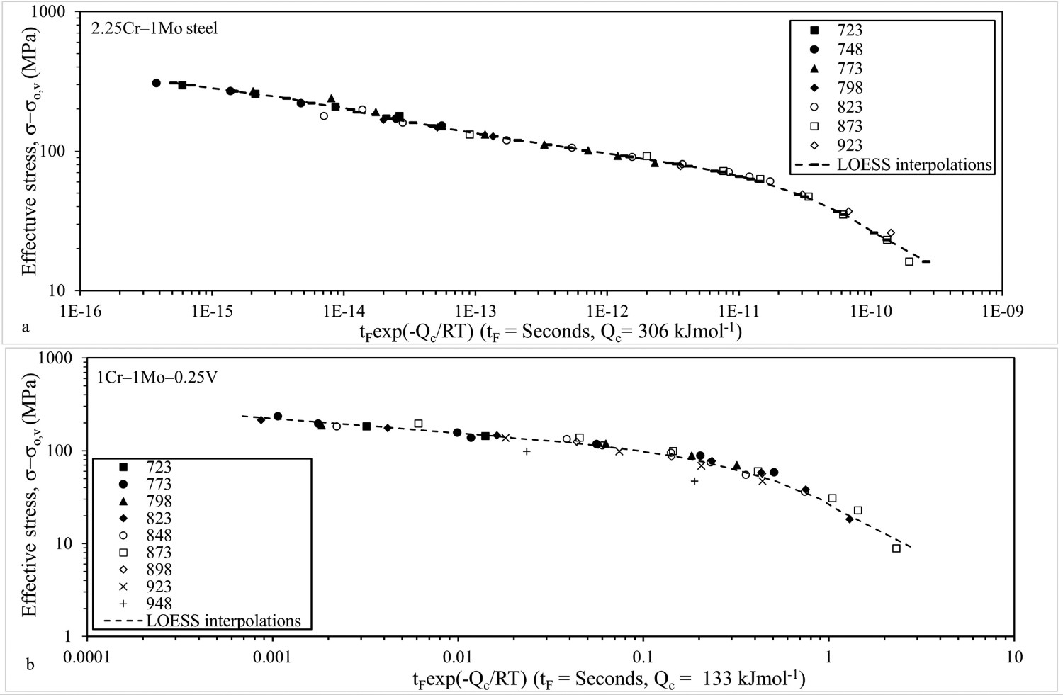
This paper makes uses of some extensive creep data sets that are currently in the public domain. NIMS Creep Data Sheet 3B &50A, published by the Japanese National Institute for Materials Science (NIMS) [22,23] provides extensive rupture data for 12 batches of 2.25Cr–1Mo steel where each batch has a different chemical composition that underwent one of four different heat treatments, details of which are given in [22]. Specimens for the tensile and creep rupture tests were taken radially from the ring-shaped samples which were removed from the virgin material. Each test specimen had a diameter of 6 mm with a gauge length of 30 mm. These specimens were tested at constant load over a wide range of conditions: 333–22 MPa and 723–923 K. In addition to minimum creep rate and time to failure measurements, values are also given of the times to attain various strains – 0.005, 0.01, 0.02 and 0.05 over a selected range of the above-mentioned test conditions. Also reported are the values of the 0.2% proof stress and the ultimate tensile strength determined from high strain tensile tests carried out at the creep temperatures for each batch of steel investigated. Failure times are averaged over all batches at each temperature, and these values are displayed in Figure 1(a).

Figure 1

Stress and temperature dependence of failure times (averaged over all batches) for (a) 2.25Cr–1Mo steel (Creep Data Sheet 3B &50A [22,23]) and (b) 1Cr–1Mo–0.25V (Creep Data Sheet 3B &50A [23,24]).

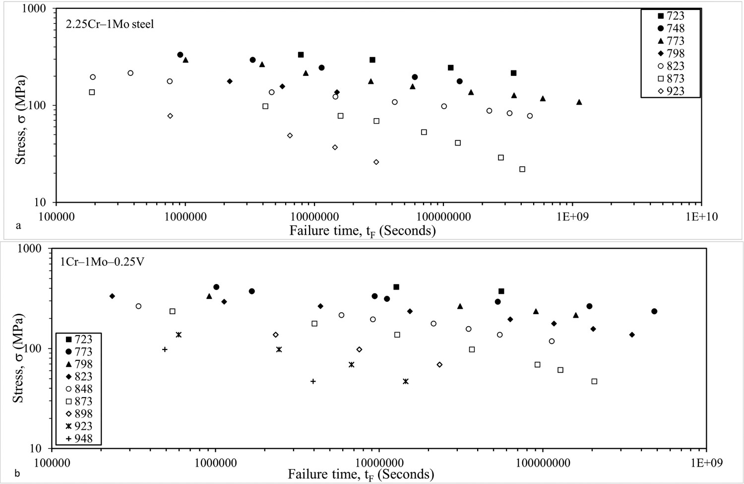
NIMS creep data sheets 9B & 50A, published by the Japanese National Institute for Materials Science (NIMS) [24,23], includes information on nine batches of tempered bainitic 1Cr–1Mo–0.25V steel, where each batch corresponded to a different heat treatment and a different chemical composition, details of which are given in [24]. Specimens for the tensile and creep rupture tests were taken radially from the ring-shaped samples which were removed from the virgin turbine rotors. Each test specimen had a diameter of 10 mm with a gauge length of 50 mm. These specimens were tested at constant load over a wide range of conditions: 412–47 MPa and 723–948 K. In addition to minimum creep rate and time to failure measurements, values are also given of the times to attain various strains – 0.005, 0.01, 0.02 and 0.05 over a selected range of the above-mentioned test conditions. Also reported are the values of the 0.2% proof stress and the ultimate tensile strength determined from high strain tensile tests carried out at the creep temperatures for each batch of steel investigated. Again, the failure times are averaged over all batches at each temperature, and these values are displayed in Figure 1(b).

In addition to these data sheets, NIMS Creep Data Sheet No. M-6 [25] is a detailed metallographic atlas, containing additional information on hardness and microstructural changes observed over time in a selection of test specimens.

Methodology

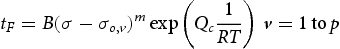
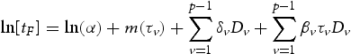
Based on Equation (3), the threshold-power law and Monkman-Grant description of time to failure at any stress and temperature combination is given by

t_{F} = B (σ - σ_{o, v})^{m} \exp (Q_{c} \frac{1}{R T}) v = 1 to p

(5a)

In Equation (5a) the threshold stress is allowed to be different at each of the p test temperatures. Again, and in relation to Equation (3), B is a new constant

.

At constant temperature this can be written as

t_{F} = α (σ - σ_{o, v})^{m}

(5b)

With

\ln (α) = \ln (B) + Q_{c} \frac{1}{R T}

(5c)

Estimating the parameters of Equation (5a) requires a combination of linear and non-linear least squares. First, the threshold stress associated with each temperature is set equal to zero. This linearises Equation (5a) (once logs are taken on both side of the equation) so that least squares can be used to estimate B, m and Q_c. These estimates will be associated with a residual sum of squares – which will be a minimum given a zero-threshold stress. Then a standard non-linear least squares procedure is used to search for better values for the threshold stresses. This search continues until, when using the estimates for the threshold stress on the last iteration of this non-linear search procedure, it is impossible to lower the residual sum of squares from a linear regression using these latest threshold stresses. In this paper, the generalised reduced gradient non-linear technique within Excel's Solver [26] is used. As such centralised derivatives are used to locate the minimum residual sum of squares.

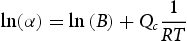
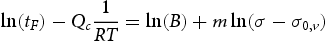
If this threshold power law model is correctly specified, the parameters B and m should be constants with respect to stress and temperature. The constancy of B and m in Equation (5a) can be tested statistically by carrying out the following regression over all temperatures

\ln [t_{F}] = \ln (α) + m (τ_{v}) + \sum_{v = 1}^{p - 1} δ_{v} D_{v} + \sum_{v = 1}^{p - 1} β_{v} τ_{v} D_{v}

(6)

where τ_ν = ln(σ−σ_0,v) and where there are p different temperatures. D_v= 1 if the test temperature corresponds to temperature T_v and zero otherwise. There is no D_v for temperature T_v = 823 K and so ln(α) is the intercept of the best fit line put through all the data points at 823 K and m its slope. In this specification, it can be shown that the values for β_v equal the values that would be obtained for m when carrying out a regression using Equation (5b) (after linearising by taking logs through both sides of the equation) applied separately to each temperature. The t statistic on δ_v and β_v then tests the null hypotheses that the intercepts and slopes of the best fit lines at other temperatures are the same as the intercept and slopes at 823 K. Statistical significance can then be measured using the p-values associated with these t statistics.

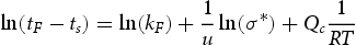
The threshold Wilshire model can be semi-linearised with respect to its unknown parameters using logs

\ln (t_{F} - t_{s}) = \ln (k_{F}) + \frac{1}{u} \ln (σ^{*}) + Q_{c} \frac{1}{R T}

(7a)

where

σ^{*} = [- \ln (\frac{σ - σ_{0, v}}{σ_{T S} - σ_{0, v}})]

(7b)

In its estimation, it is again assumed that Q_c is a constant with respect to test conditions and threshold stress only varies with temperature. To estimate the parameters of Equations (7), the threshold stress associated with each temperature are first set equal to zero. Least squares can be used to estimate k_F, u and Q_c. These estimates will be associated with a residual sum of squares – which will be a minimum given a zero-threshold stress. Then Excel's Solver [26] is used to find better values for the threshold stresses in the same way as that described for the power law model.

In either of these models, the joint significance of the threshold stresses can be tested using the F test given by Equation [A13] in Appendix 2. The ability of Equations (5) and (7) to adequately describe failure times can be assessed using the RESET test given in Appendix 1. It can also be assessed using the performance statistics discussed in more detail in Appendix 1.

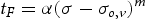
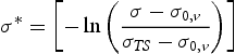
Another approach to dealing with any observed variation in m and u is to accept that these models are an imperfect explanation of minimum creep rates and failure times. That is, the model is only a realistic explanation of creep over a reduced range of test conditions. One way to implement this is to have an estimation procedure that only considers test conditions local to the test condition of interest. Once repeated for all test conditions of interest, this estimation procedure will then reveal the nature of the variation in u and m with the test conditions and so could reveal more information on changing creep mechanisms. One such estimation procedure is the locally weighted scatterplot smoothing (LOESS) curve first proposed by Cleveland [21]. Here data points around a chosen test condition are weighted with points further away from this chosen test condition being given less weight in a standard least squares estimation (i.e. weighted least squares are used). A zero weight is then used for conditions beyond a selected band width. This process is then repeated for all stresses and temperatures revealing different values for the model parameters B, m, k_F and u at each test condition. These can then be used to make interpolations and/or extrapolations. To achieve this, the power threshold and Wilshire models are rewritten as

\begin{aligned} \ln (t_{F}) - Q_{c} \frac{1}{R T} & = \ln (B) + m \ln (σ - σ_{0, v}) \end{aligned}

(8a)

\begin{aligned} \ln (t_{F} - t_{s}) - Q_{c} \frac{1}{R T} & = \ln (k_{F}) + \frac{1}{u} \ln (σ^{*}) \end{aligned}

(8b)

More details of this technique are provided in Appendix 2, where it is further assumed that Q_c is a constant – so that only the values for parameters B, m, u and k_F are dependent on test conditions. The threshold stress only varies with temperature.

Results and discussion

Non-linear least squares estimation of the threshold power law model

2.25Cr–1Mo steel

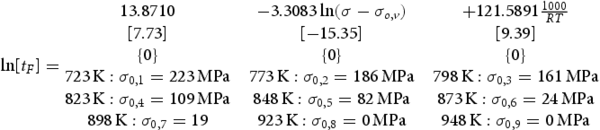
Equation (9) shows the results of estimating Equation (5b) using the non-linear search procedure described in the methodology section above

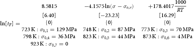
\begin{aligned} \ln [t_{F}] = \begin{matrix} 8.5815 & - 4.1575 \ln (σ - σ_{o, v}) & + 178.4017 \frac{1000}{R T} \\ [6.40] & [- 23.23] & [16.29] \\ {0} & {0} & {0} \\ 723 K : σ_{0, 1} = 129 MPa & 748 K : σ_{0, 2} = 87 MPa & 773 K : σ_{0, 3} = 70 MPa \\ 798 K : σ_{0, 4} = 36 MPa & 823 K : σ_{0, 5} = 44 MPa & 873 K : σ_{0, 6} = 4 MPa \\ 923 K : σ_{0, 7} = 0 \end{matrix} \end{aligned}

(9)

where the square brackets contain the t values associated with the null hypothesis that the parameter value above it are zero, and the numbers in curly brackets the p-value associated with this t test (and so give the probability of this null hypothesis being true). There are a number of observations around Equation (9) that indicate this representation of creep is reasonable. First, a positive threshold stress is observed at all temperatures except at 923 K. The joint statistical significance of these threshold stresses was tested using the F test given by Equation (A13) in Appendix 2. This F value comes out at 7.4, which is statistically significant even at the 1% significance level. Thus, while the threshold stress may not be present at all temperatures, there are threshold stresses that are strongly dependent on temperature – being highest at the lowest temperatures. Second, the R² value for this model is 93.24%, which is quite reasonable given the stochastic nature of creep.

\begin{aligned} ln t_{F} & = \begin{matrix} 11.95 & - 2.34 D_{1} & - 0.16 D_{2} & - 4.78 D_{3} & + 4.01 D_{4} & - 5.57 D_{6} & - 6.76 D_{7} \\ [0] & [0.03] & [0.96] & [0.02] & [0.71] & [0] & [0.02] \\ - 4.99 τ_{5} & + 0.62 τ_{1} D_{1} & + 0.17 τ_{2} D_{2} & + 1.17 τ_{3} D_{3} & - 0.72 τ_{4} D_{4} & + 1.49 τ_{6} D_{6} & + 1.62 τ_{7} D_{7} \\ [0] & [0.49] & [0.81] & [0.01] & [0.75] & [0] & [0.03] \end{matrix} \end{aligned}

(10)

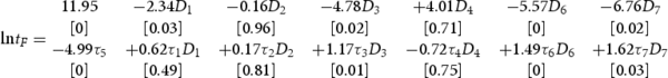
and the p-values in parenthesis clearly show that the stress exponent m and intercept term in Equation (9) are not really constant with respect to all temperatures. The value for m at 823 K is −4.99, while at 773 K it is −4.99 + 1.17 and this difference is statistically significant at the 5% significance level. The value for the intercept (α) at 823 K is 11.95, while at 773 K it is 11.95-4.78 and this difference is again statistically significant at the 5% significance level. As well as this, m at 873 and 923 K are statistically different from the value at 823 K. Equation (10) suggests then that m varies between −3 and −5 –values that are consistent with dislocation climb. The lack of constancy in m is visualised in Figure 2(a).

Figure 2

Dependency of the temperature adjusted average failure times (calculated using Q_c= 178 kJ mol⁻¹ in the threshold power law model) for (a) 2.25Cr–1Mo and (b) 1Cr–1Mo–0.25V steels.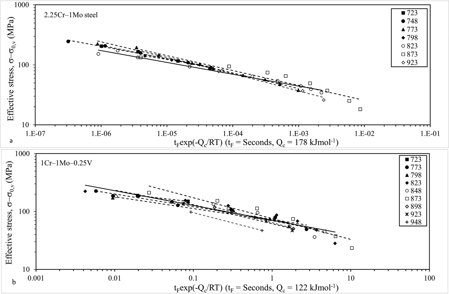

In addition, when the squared predictions obtained from Equation (9) are added as another variable to Equation (9), the resulting RESET test gave a p-value of 0.003 for the null hypothesis of no misspecification, thus suggesting this threshold power law model is statistically mis-specified at the 1% significance level. This misspecification can be seen in Figure 2(a), which plots t_F exp[178(1000/RT)] against (σ−σ_0,v) revealing data points that define a curve rather than a line.

The top half of Table 1 gives further evidence that while not perfect, the threshold power law model is a reasonable but mis-specified description of the creep failure times. The Z statistic is unacceptable high (>4) at 823 and 873 K. The MPSE is reasonable at most temperatures – except at 873 K. But on the plus side nearly 70% of this error is random in nature. Indeed the proportion of the MPSE that is random in nature is quite high (above 20%) except at 798 K.

Table 1

Interpolative performance of the threshold power law model when applied to two different low-alloy steels.

	948 K	923 K	898 K	873 K	848 K	823 K	798 K	773 K	748 K	723 K
		2.25Cr–1Mo steel
Z	–	3.4	–	13.8	–	4.9	2.0	2.3	2.4	1.6
MPSE	–	31.7	–	105.7	–	38.7	4.7	10.3	9.7	2.3
RMPSE	–	5.6	–	10.3	–	6.2	2.2	3.2	3.1	1.5
U_M	–	46.3	–	14.5	–	11.1	1.8	13.7	7.6	1.5
U_R	–	32.3	–	16.1	–	53.5	96.4	39.3	63.5	20.9
U_D	–	21.4	–	69.4	–	35.4	1.8	47.0	28.9	77.6
		1Cr–1Mo–0.25V steel
Z	1.9	2.1	2.0	8.9	7.2	10.7	9.5	6.5	–	3.7
MPSE	146.9	7.1	5.4	8.4	51.6	75.1	59.9	50.0	–	12.9
RMPSE	12.1	2.7	2.3	9.2	7.2	8.7	7.7	7.1	–	3.6
U_M	98.0	17.7	10.5	26.8	2.3	1.5	4.8	9.8	–	1.3
U_R	2.0	26.7	85.5	36.5	0.7	1.1	47.4	51.1	–	98.7
U_D	0.0	55.6	4.0	36.7	97.0	97.4	47.8	39.1	–	0.0

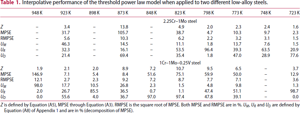
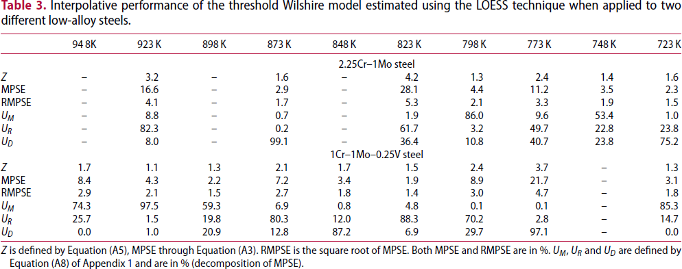
Z is defined by Equation (A5), MPSE through Equation (A3). RMPSE is the square root of MPSE. Both MPSE and RMPSE are in %. U_M, U_R and U_D are defined by Equation (A8) of Appendix 1 and are in % (decomposition of MPSE).

1Cr–1Mo–0.25V steel

Equation (11) shows the results of estimating the threshold power law model for 1Cr–1Mo–0.25V steel

\begin{aligned} \ln [t_{F}] & = \begin{matrix} 13.8710 & - 3.3083 \ln (σ - σ_{o, v}) & + 121.5891 \frac{1000}{R T} \\ [7.73] & [- 15.35] & [9.39] \\ {0} & {0} & {0} \\ 723 K : σ_{0, 1} = 223 MPa & 773 K : σ_{0, 2} = 186 MPa & 798 K : σ_{0, 3} = 161 MPa \\ 823 K : σ_{0, 4} = 109 MPa & 848 K : σ_{0, 5} = 82 MPa & 873 K : σ_{0, 6} = 24 MPa \\ 898 K : σ_{0, 7} = 19 & 923 K : σ_{0, 8} = 0 MPa & 948 K : σ_{0, 9} = 0 MPa \end{matrix} \end{aligned}

(11)

Again, there are several observations around Equation (11) that indicate this representation of creep is reasonable for this material. First, a positive threshold stress is observed at all temperatures except above 898 K. The F test for the joint significance of these threshold stresses comes out at 6.3, which again is statistically significant even at the 1% significance level. Thus, once again there are threshold stresses that are strongly dependent on temperature. Compared to 2.25Cr–1Mo steel, these threshold stresses are much larger, however. Second, the R² value for this model is reasonably high at 86.2%. Thirdly, the estimation of Equation (6) yielded

\begin{aligned} ln t_{F} & = \begin{matrix} 14.54 & + 15.04 D_{1} & + 4.07 D_{2} & + 4.80 D_{3} & - 1.16 D_{5} & - 3.47 D_{6} & - 3.34 D_{7} & - 2.36 D_{8} & - 3.91 D_{9} \\ [0] & [0.52] & [0.23] & [0.28] & [0.71] & [0.17] & [0.56] & [0.60] & [0.54] \\ - 3.44 τ_{5} & - 2.95 τ_{1} D_{1} & - 0.91 τ_{2} D_{2} & - 1.12 τ_{3} D_{3} & + 0.26 τ_{5} D_{5} & + 0.88 τ_{6} D_{6} & + 0.75 τ_{7} D_{7} & + 0.48 τ_{8} D_{8} & + 0.61 τ_{9} D_{9} \\ [0] & [0.52] & [0.20] & [0.25] & [0.70] & [0.11] & [0.56] & [0.63] & [0.68] \end{matrix} \end{aligned}

(12)

and the p-values in parenthesis clearly show that the stress exponent m and intercept term in Equation (11) are constant with respect to all temperatures at the 10% significance level (but at the 5% significance level, m may be different at 873 K compared to 823 K). The value for m at 823 K is −3.44, while at 873 K it is −3.44 + 0.88 and this difference is not statistically significant at the 10% significance level. The value for the intercept (α) at 823 K is 14.54 and at the 10% significance level the intercept is no different at any other temperature. Equation (12) suggests then that m is around −3.44 – a value that is consistent with dislocation climb. The near constancy in m is visualised in Figure 2(b). Fourthly, when the squared predictions obtained from this equation are added as another variable to Equation (11) the resulting RESET test gave a p-value of 0.053 for the null hypothesis of no misspecification, Thus suggesting this threshold power law model is not mis-specified using a 5% significance level (but it is at the 1% significance level).

However, there are also some features of this model that suggest it is mis-specified or at least an imperfect descriptor of the observed failure times, First, the estimated activation energy of around 122 kJ mol⁻¹ is well below the activation energy for self-diffusion quoted by Scharning and Wilshire [8] (of around 300 kJ mol⁻¹ for this material). Second, the bottom half of Table 1 gives further evidence for this material that the threshold power law model is far from an ideal description of the creep failure times. At all temperatures, the Z statistic is unacceptable high (>4) at 773–873 K. At these temperatures the MPSE is high with values between 8% and 60%. The random component of this MPSE remains very low at 948, 898 and 723 K.

Possible explanations for varying stress exponent

The reason for a smaller slope at high temperatures could be down to the fact that some specimens tested at these temperatures all remained exposed for the longest periods of time because they were conducted at the lowest stresses within the test matrix. An inspection of some of the images of the failed test specimens in creep data sheet 3B [22] at these temperatures and long exposures revealed the presence of an oxidised surface that could weaken its load bearing strength. Further, the NIMS Metallographic Atlas [25] reveals that the received bainitic regions degrades to Ferrite and Molybdenum carbide particles, with very coarse carbides along grain boundaries. Both of these phenomena would result in faster creep rates and creep lives that are substantially shorter in tests of long duration at 873 K and above, than would be expected by direct extrapolation of the best fit lines seen in Figure 2(a,b) at the lower temperatures That is, it would result in the bending of the curve seen in the figures at the long exposure present at these high temperatures and lower stresses. The second of these two explanations would then be consistent with the presence of a threshold stress below 873 K – with carbide coarsening at the high temperatures removing the need for a minimum stress required for dislocations to move.

Explanation for the presence of threshold stresses

The presence of a threshold stress and its dependence on temperature could reflect the fact that for this data set, the longest exposed test specimens are at the highest two temperatures (due to the low stresses), where as noted above, noticeable carbide coarsening takes place. This will weaken the barriers to dislocation movement and so remove the presence of a minimum or threshold stress required for dislocation movement. Consequently, the estimated threshold stresses are at 873 and 923 K either zero or very close to it. Alternatively, the presence of large threshold stresses at the lowest temperatures may be the result of lower thermal energies making creep more stress-dependent – i.e. requiring a minimum stress before barriers to dislocation movement can be overcome. This minimum is larger the lower the thermal energy present – the lower is the temperature.

LOESS estimation of the threshold power law model

2.25Cr–1Mo steel

Figure 3(a,b) shows some results from using this LOESS procedure to estimate the parameters of Equation (8a) for 2.25Cr–1Mo data. Both B and m follow very similar patterns showing a very strong dependency on test conditions. At temperatures of 823 K and above and with stresses less than around 150 MPa, ln(B) increases with stress and m decreases with stress. Between a stress of around 150 and 250 MPa both these parameters are broadly constant at temperatures below 823 K and for higher stresses ln(B) starts to increase and m decrease with stress.

Figure 3

Dependency of (a) ln(B) and (b) m in Equation (8a) on test conditions for 2.25Cr–1Mo steel.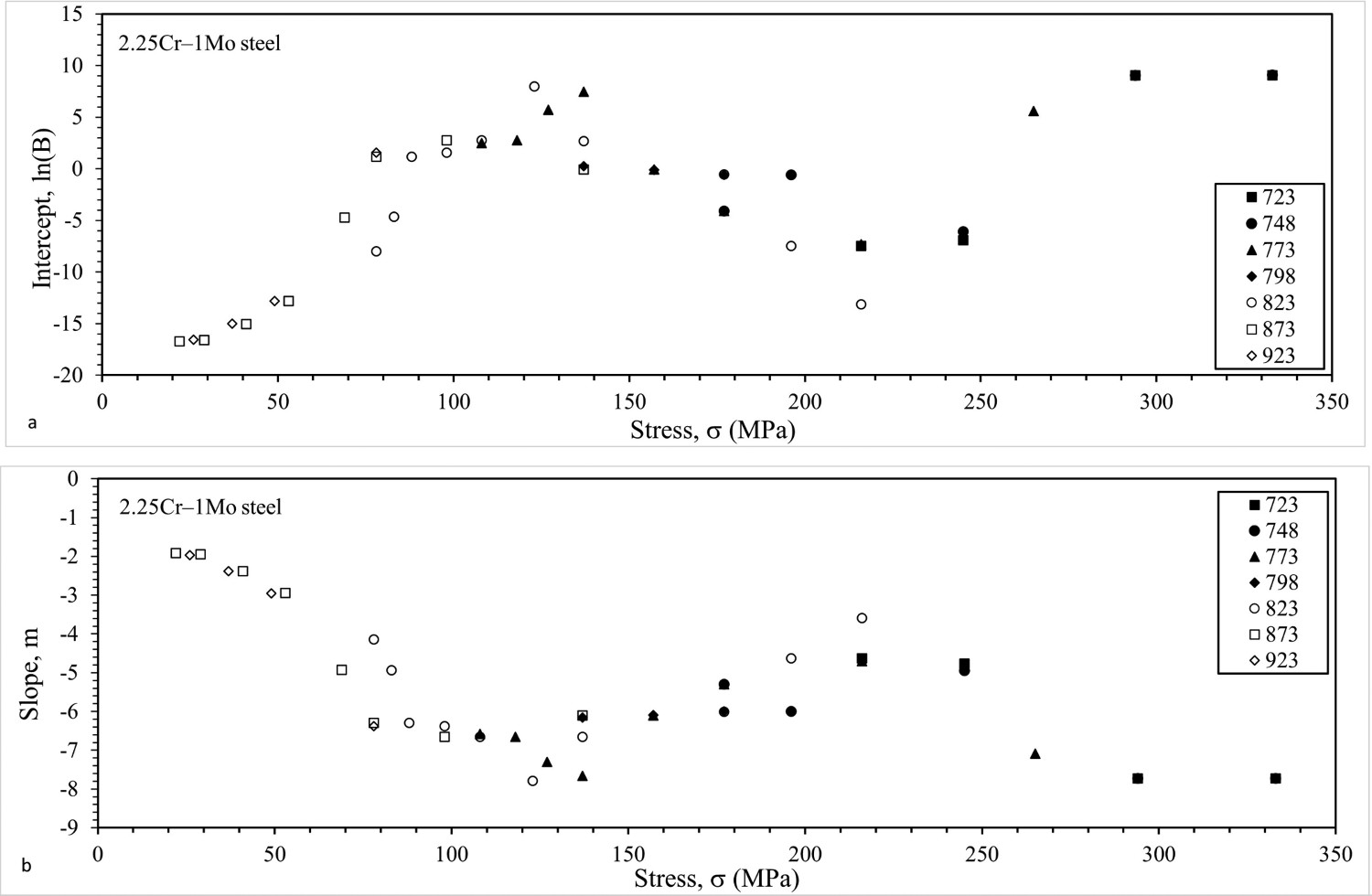

The value for Q_c was estimated at 306 kJ mol⁻¹, again rather on the large side for this material, and the threshold stresses were estimated at

\begin{array}{l} 723 K : σ_{0, 1} = 37 MPa; 748 K : σ_{0, 2} = 25 MPa; \\ 773 K : σ_{0, 3} = 26 MPa; \\ 798 K : σ_{0, 4} = 10 MPa; 823 K : σ_{0, 5} = 17 MPa \\ 873 K : σ_{0, 6} = 6 MPa; 923 K : σ_{0, 7} = 0 MPa \end{array}

which are much smaller in value than those obtained in Equation (9). Nevertheless, they are jointly significantly different from zero at the 1% significance level with a F statistic value of 13.6. Figure 4(a) then plots the interpolated time-adjusted failure times obtained by substituting into Equation (8a) the values for ln(B) and m shown in Figure 3(a,b), together with the Q_c and threshold stress values are shown above. Compared to Figure 2(a), an improvement is noticeable in terms of reduced scatter in the data around a smooth continuous interpolation curve that represents this data quite well. This is further seen in the statistics shown in the top half of Table 2. Compared to the threshold power law model estimated via non-linear least square, the Z values are lower at all temperatures – especially at 873 K where this LOESS estimated model is far superior in performance. All the Z values are also much lower than the critical value of 4. The MSPE is also considerably lower at all temperatures (except at 773 K where they are the same). In terms of how much of this MPSE is random in nature there is a mixed picture. The LOESS estimated model has more random interpolative error at 873, 823 and 798 K, but lower a lower random component at other temperatures.

Figure 4

Temperature-adjusted failure times as a function of stress together with LOESS interpolations obtained using Equation (8a) and parameter values in Figures 3 and 6(a,b), for (a) 2.25Cr–1Mo and (b) 1Cr–1Mo–0.25V–steels.

Table 2

Interpolative performance of the threshold power law model estimated using the LOESS technique when applied to two different low-alloy steels.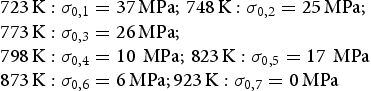

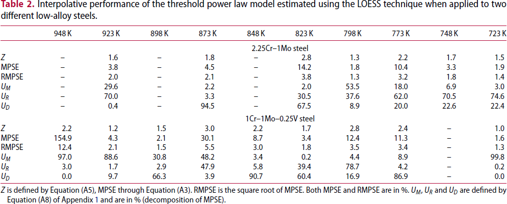
	948 K	923 K	898 K	873 K	848 K	823 K	798 K	773 K	748 K	723 K
	2.25Cr–1Mo steel
Z	–	1.6	–	1.8	–	2.8	1.3	2.2	1.7	1.5
MPSE	–	3.8	–	4.5	–	14.2	1.8	10.4	3.3	1.9
RMPSE	–	2.0	–	2.1	–	3.8	1.3	3.2	1.8	1.4
U_M	–	29.6	–	2.2	–	2.0	53.5	18.0	6.9	3.0
U_R	–	70.0	–	3.3	–	30.5	37.6	62.0	70.5	74.6
U_D	–	0.4	–	94.5	–	67.5	8.9	20.0	22.6	22.4
	1Cr–1Mo–0.25V steel
Z	2.2	1.2	1.5	3.0	2.2	1.7	2.8	2.4	–	1.0
MPSE	154.9	4.3	2.1	30.1	8.7	3.4	12.4	11.3	–	1.6
RMPSE	12.4	2.1	1.5	5.5	3.0	1.8	3.5	3.4	–	1.3
U_M	97.0	88.6	30.8	48.2	3.4	0.2	4.4	8.9	–	99.8
U_R	3.0	1.7	2.9	47.9	5.8	39.4	78.7	4.2	–	0.2
U_D	0.0	9.7	66.3	3.9	90.7	60.4	16.9	86.9	–	0.0

This is all visualised in Figure 5(a). The solid curves show the interpolations of time to failure at each stress and consistent with the statistics in Table 2, the interpolations look poorest at 948 K.

Figure 5

Failure times as a function of stress together with this LOESS interpolations obtained using Equation (8a) for (a) 2.25Cr–1Mo and (b) 1Cr–1Mo–0.25V steels.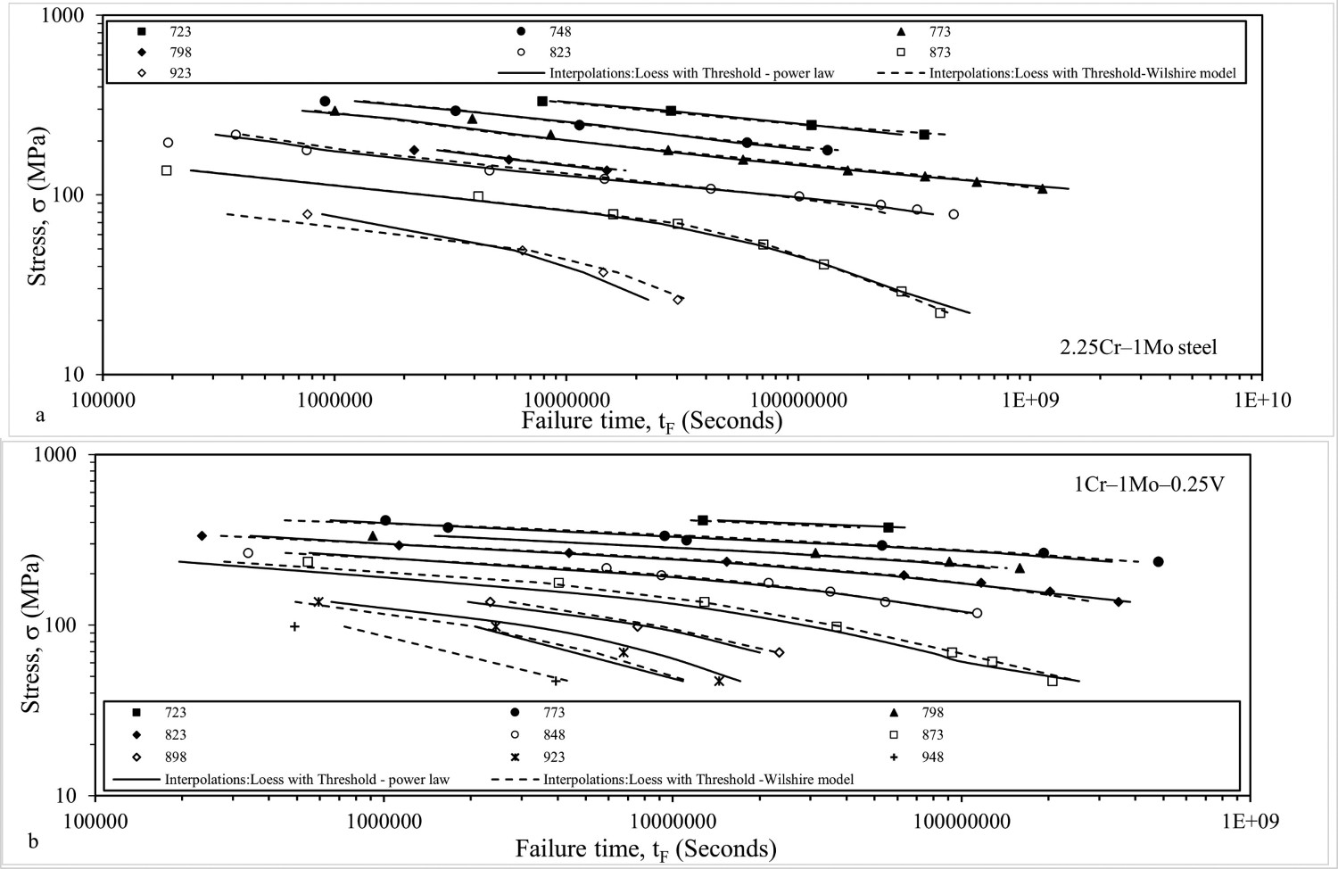

1Cr–1Mo–0.25V steel

Figure 6(a,b) shows some results from using this LOESS procedure on 1Cr–1Mo–0.25V steel. Both B and m are strongly dependent on test conditions but in a more straightforward way than for 2.25Cr–1Mo steel. Up to around 325 MPa, ln(B) increases with stress and m decreases with stress. At temperatures of 823 K and above with stress less than around 150 MPa ln(B) increases with stress and m decreases with stress. Temperature then shifts the dependency in an almost parallel fashion. Above 325 MPa and for temperatures below 798 K these parameters remain constant with respect to stress.

Figure 6

Dependency of (a) ln(B) and (b) m in Equation (8a) on test conditions for 1Cr–1Mo–0.25V steel.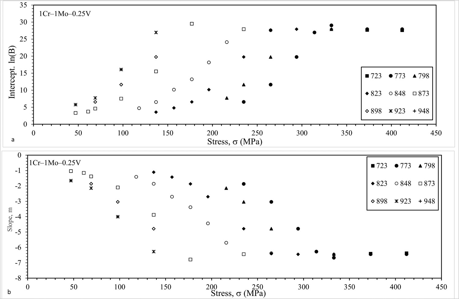

The value for Q_c was estimated at 133 kJ mol⁻¹, again unrealistically small for this material, and the threshold stresses were estimated at

\begin{aligned} 723 K : σ_{0, 1} & = 229 MPa; 773 K : σ_{0, 2} = 176 MPa; \\ 798 K : σ_{0, 3} & = 146 MPa; 823 K : σ_{0, 4} = 119 MPa; \\ 848 K : σ_{0, 5} & = 82 MPa; 873 K : σ_{0, 6} = 38 MPa; \\ 898 K : σ_{0, 7} & = 12 MPa; 923 K : σ_{0, 8} = 0 MPa; \\ 948 K : σ_{0, 9} & = 0 MPa \end{aligned}

which are much the same in value as in Equation (11). Further, they are jointly significantly different from zero at the 5% significance level with an F statistic value of 2.9. Figure 4(b) then plots the interpolated time-adjusted failure times obtained by substituting into Equation (8a) the values for ln(B) and m shown in Figure 6(a,b) together with the Q_c and threshold stress values shown above. Compared to Figure 2(b), an improvement is noticeable in terms of reduced scatter in the data around a smooth continuous interpolation curve that represents these data quite well. The scatter is not as small however as in the case of 2.25Cr–1Mo steel. This is also apparent in the statistics shown in the bottom half of Table 2. Compared to the threshold power law model estimated via non-linear least squares (Table 1), the Z values are lower at all temperatures except 948 K – and at 848 K and above this LOESS estimated model is far superior in performance. All the Z values are also much lower than the critical value of 4. The MSPE is also considerably lower at all temperatures except at 948 K. In terms of how much of this MPSE is random in nature there is a mixed picture. This LOESS estimated model has more random interpolative error at 898 and 773 K. This is all visualised in Figure 5(b). The solid curves show the interpolations of time to failure at each stress using LOESS and are consistent with the statistics in Table 2 – the interpolations look poorest at 948 and 873 K.

LOESS estimation of the threshold Wilshire model

2.25Cr–1Mo steel

Figure 7(a,b) contain the values for ln(k_F) and 1/u of Equation (8b) found at each test condition using LOESS. Both ln(k_F) and 1/u show a strong dependency on test conditions. At temperatures of 823 K and above with stress levels less than around 125 MPa, ln(k_F) decreases with stress and 1/u increases with stress. Then at higher stresses and lower temperatures, ln(k_F) is broadly constant with respect to stress, while 1/u shows a slight tendency to decline with stress.

Figure 7

Dependency of (a) ln(k_F) and (b) 1/u in Equations (8b) on test conditions for 2.25Cr–1Mo steel.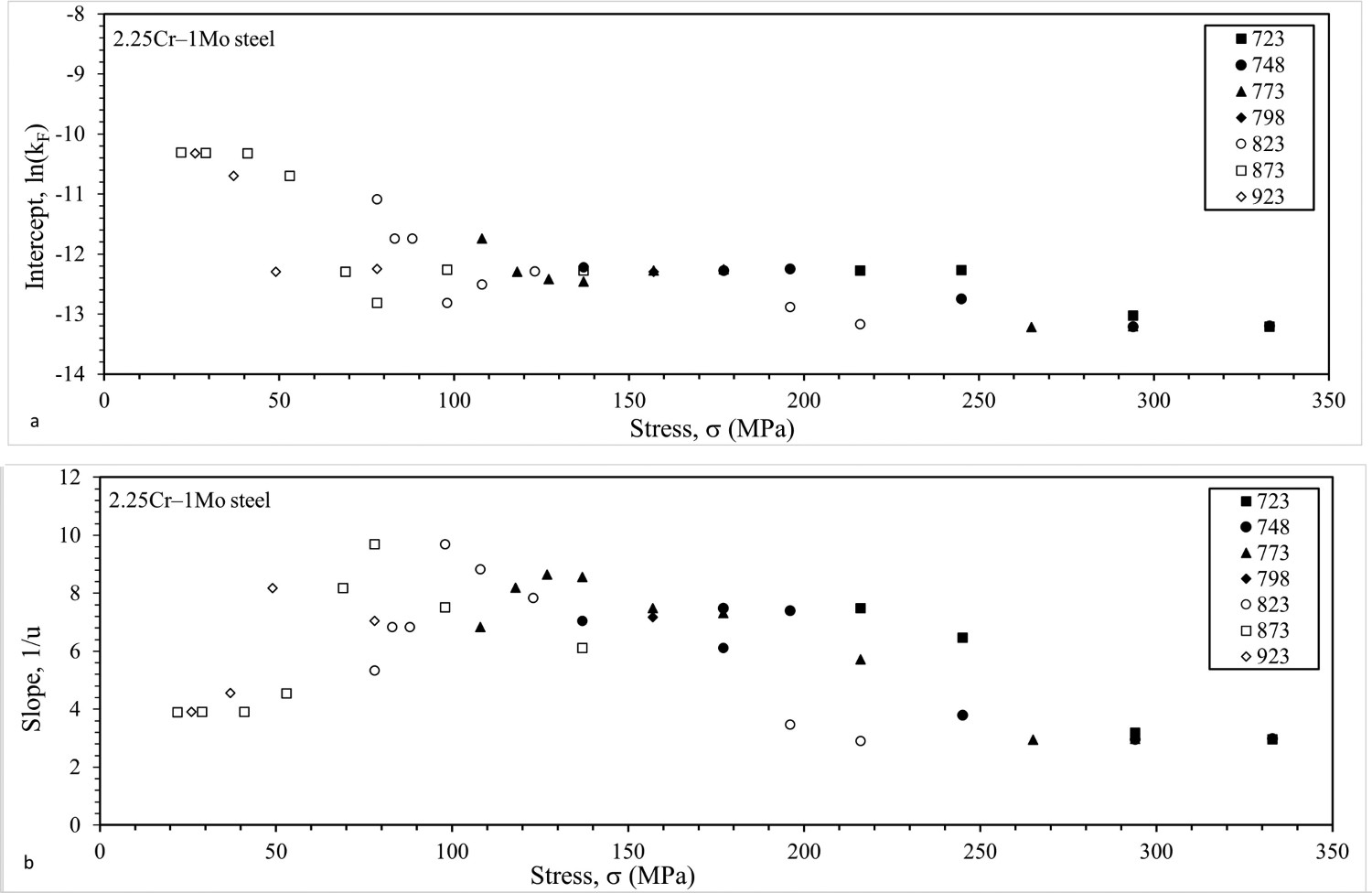

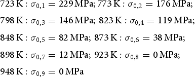
The value for Q_c was estimated at 190 kJ mol⁻¹, which is closer to the value of 230 kJ mol⁻¹ reported by Wilshire and Whittaker [27] than the value obtained above using LOESS or non-linear least squares on the threshold power law model. The threshold stresses were estimated as

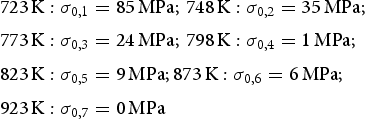
\begin{aligned} 723 K : σ_{0, 1} & = 85 MPa; 748 K : σ_{0, 2} = 35 MPa; \\ 773 K : σ_{0, 3} & = 24 MPa; 798 K : σ_{0, 4} = 1 MPa; \\ 823 K : σ_{0, 5} & = 9 MPa; 873 K : σ_{0, 6} = 6 MPa; \\ 923 K : σ_{0, 7} & = 0 MPa \end{aligned}

It appears that the creep model used has only a minimal effect on the estimated threshold stress. The only noticeable difference appears at 723 K where the Wilshire model has a threshold stress about twice as large as in the threshold power law model. These threshold stresses are jointly significantly different from zero at the 1% significance level with and F statistic value of 7.05.

Figure 8(a) then plots the interpolated time-adjusted failure times obtained by substituting into Equation (8b) the values for ln(k_F) and 1/u shown in Figure 7(a,b) together with the Q_c and threshold stress values shown above. Compared to Figure 4(a), there appears to be more scatter around the model's interpolated values, especially at higher stresses, and the fit is not so good at 823 K in the LOESS estimated threshold Wilshire model. In the threshold power law model deviations from a straightish line occurs only once, while in the threshold Wilshire model this happens twice. This is further seen in the statistics shown in the top half of Table 3. Compared to the threshold power law model estimated via LOESS (Table 2), the Z values are about the same or a little higher depending on the temperature – especially at 823 K where the LOESS estimated threshold Wilshire model is far inferior in performance. All the Z values are also the same or much lower than the critical value of 4. The same picture holds for the MSPE. The LOESS estimated threshold Wilshire model has more random interpolative error at all of the temperatures except at 823 K compared to the LOESS estimated threshold power law model.

Figure 8

Temperature-adjusted failure times as a function of stress together with the LOESS interpolations obtained using Equations (8b) for (a) 2.25Cr–1Mo and (b) 1Cr–1Mo–0.25V steels.

Table 3

Interpolative performance of the threshold Wilshire model estimated using the LOESS technique when applied to two different low-alloy steels.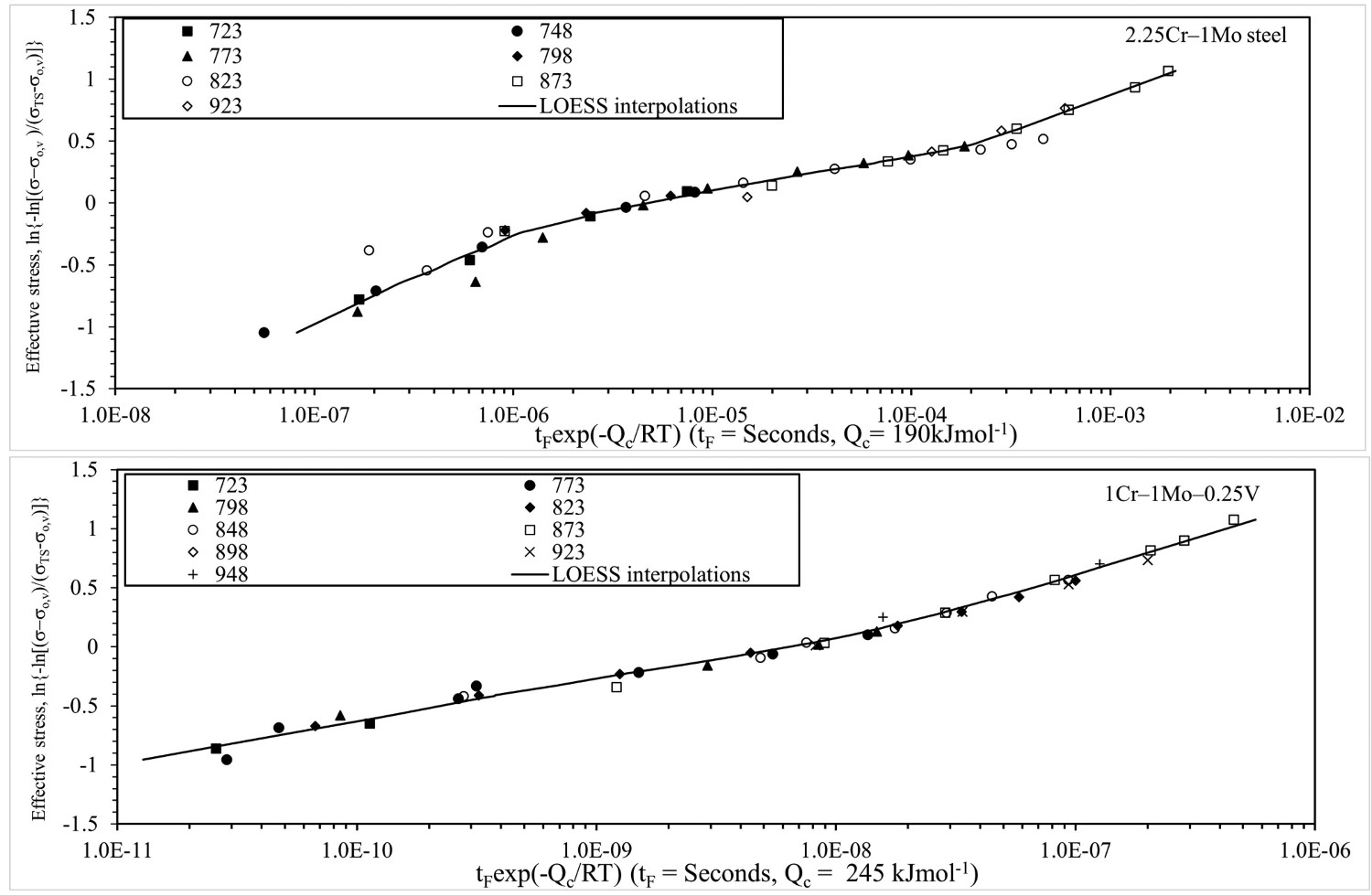

	94 8K	923 K	898 K	873 K	848 K	823 K	798 K	773 K	748 K	723 K
	2.25Cr–1Mo steel
Z	–	3.2	–	1.6	–	4.2	1.3	2.4	1.4	1.6
MPSE	–	16.6	–	2.9	–	28.1	4.4	11.2	3.5	2.3
RMPSE	–	4.1	–	1.7	–	5.3	2.1	3.3	1.9	1.5
U_M	–	8.8	–	0.7	–	1.9	86.0	9.6	53.4	1.0
U_R	–	82.3	–	0.2	–	61.7	3.2	49.7	22.8	23.8
U_D	–	8.0	–	99.1	–	36.4	10.8	40.7	23.8	75.2
	1Cr–1Mo–0.25V steel
Z	1.7	1.1	1.3	2.1	1.7	1.5	2.4	3.7	–	1.3
MPSE	8.4	4.3	2.2	7.2	3.4	1.9	8.9	21.7	–	3.1
RMPSE	2.9	2.1	1.5	2.7	1.8	1.4	3.0	4.7	–	1.8
U_M	74.3	97.5	59.3	6.9	0.8	4.8	0.1	0.1	–	85.3
U_R	25.7	1.5	19.8	80.3	12.0	88.3	70.2	2.8	–	14.7
U_D	0.0	1.0	20.9	12.8	87.2	6.9	29.7	97.1	–	0.0

This is all visualised in Figure 5(a). The dashed curves show the interpolated time to failures at each stress for the threshold Wilshire model. Consistent with the statistics in Tables 2 and 3, the threshold Wilshire interpolations look better than the threshold power law model at 873 K but worse at 823 K.

1Cr–1Mo–0.25V steel

Figure 9(a,b) contains the values for ln(k_F) and 1/u found at each test condition. Both ln(k_F) and 1/u show a very strong dependency on test conditions. At temperatures of 848 K and above and with stresses less than around 250 MPa, ln(k_F) decreases with stress and 1/u increases with stress. Then at higher stresses and lower temperatures ln(k_F) and 1/u are broadly constant with respect to stress.

Figure 9

Dependency of (a) ln(k_F) and (b) 1/u in Equations (8b) on test conditions for 1Cr–1Mo–0.25V steel.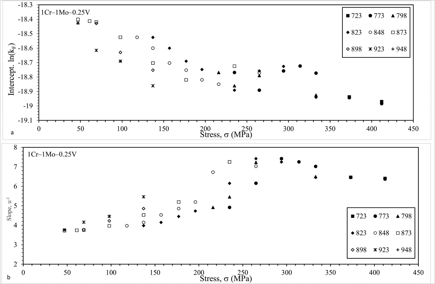

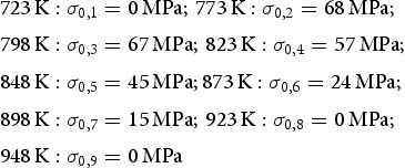
The value for Q_c was estimated at 245 kJ mol⁻¹, again rather on the small side for this material, and the threshold stresses were estimated at

\begin{aligned} 723 K : σ_{0, 1} & = 0 MPa; 773 K : σ_{0, 2} = 68 MPa; \\ 798 K : σ_{0, 3} & = 67 MPa; 823 K : σ_{0, 4} = 57 MPa; \\ 848 K : σ_{0, 5} & = 45 MPa; 873 K : σ_{0, 6} = 24 MPa; \\ 898 K : σ_{0, 7} & = 15 MPa; 923 K : σ_{0, 8} = 0 MPa; \\ 948 K : σ_{0, 9} & = 0 MPa \end{aligned}

For this material, model selection seems to make a big difference to the estimated threshold stress at temperature at or below 848 K. At higher temperatures the values are very similar. Unusually, the estimated threshold stress at 723 K is zero – but this may reflect the small number of observations at this temperature (just two data points). Nevertheless, these stresses are jointly significantly different from zero at the 5% significance level with and F statistic value of 2.12. Figure 8(b) then plots the interpolated temperature-adjusted failure times obtained by substituting into Equation (8b) the values for ln(k_F) and 1/u shown in Figure 9(a,b), together with the Q_c and threshold stress values shown above. Compared to Figure 4(b), there appears to be less scatter around the model's interpolated values, and the relationship with stress appears more straightforward than for 2.25Cr–1Mo steel. There also appears to be less scatter around this models interpolated values and the relationship with stress appears more straightforward compared to the LOESS estimated threshold power law model. This is further seen in the statistics shown in the bottom half of Table 3. Compared to the threshold power law model estimated via LOESS (Table 2), the Z values are about the same or a little smaller depending on the temperature (except at 773 K where it is a little higher). All the Z values are also much lower than the critical value of 4. The same picture holds for the MSPE. The LOESS estimated threshold Wilshire model has more random interpolative error at temperatures of 873, 798 and 773 K compared to the LOESS estimated threshold power law model. The opposite is true at other temperatures.

This is all visualised in Figure 5(b). The dashed curves show the interpolated time to failure at each stress for the threshold Wilshire model. Consistent with the statistics in Tables 2 and 3 the threshold Wilshire interpolations look better than the threshold power law model at all temperatures except 923 and 898 K.

Both the threshold power law and Wilshire models gave unreasonable values for the activation energy irrespective of whether it was estimated via LOESS or non-linear least squares. Despite this shortcoming, estimation via LOESS resulted in improved interpolative performance. The improved interpolations come about because interpolations are based on restricted observations around the test condition of interest when using LOESS. But the values for Q_c still suggest the models are miss specified. These unrealistic Q_c values likely come from forcing Q_c to be a constant over all test conditions in the models used in the paper. The possibility of an activation energy being dependent on test conditions would fit well with the LOESS methodology and warrants future research.

Conclusion

This paper presented an investigation into the significance of a threshold stress within a power law and the Wilshire models. For both materials that were studied in this paper, a statistically significant threshold stress was found and that this stress varied with temperature. The choice of creep model had a much smaller impact on the estimated threshold stress compared to the estimation technique – LOESS vs non-linear least squares. The values for the threshold stress at each temperature in the LOESS estimated Wilshire model were much closer to the typical operating stress for these materials.

The use of Z together with its decomposition overcomes the problem of using Z to assess interpolative performance (large Z values are not necessarily bad if all the interpolation errors are random).

When the LOESS estimation procedure was applied to the threshold power law model an improved interpolative capability was observed when compared to that model estimated via non-linear least squares. The scatter in the temperature-adjusted failure times ware dramatically reduced yielding a smooth well defined but non-linear relationship with stress.

When the LOESS estimation procedure was applied to a threshold-modified Wilshire model an improved interpolative capability (as measured by Z and MPSE) compared to the threshold power law model was observed at nearly all temperatures for both for 2.25Cr–1Mo and 1Cr–1Mo–0.25V steel. In terms of how much of this MPSE was random in nature, a more mixed picture emerged. For 2.25Cr–1Mo steel, the LOESS estimated threshold Wilshire model produced more random interpolation errors at all but one temperature, while for 1Cr–1Mo–0.25V steel the LOESS estimated threshold power law model performed better in around two thirds of the temperatures studied.

The estimated activation energy was still unreasonable in – especially for 1Cr–1Mo–0.25V steel – coming out at just 190 kJ mol⁻¹. This may be an indication that the creep models used are mis-specified.

The implications of including a threshold stress for extrapolative capability remain to be assessed. In particular, the stability of the estimated threshold stress when using failure times of up to 10,000 h or less remains to be quantified and should form part of any future research efforts.

Footnotes

Disclosure statement

No potential conflict of interest was reported by the author(s).

Data availability statement

All data used in this publication are in the public domain [22–].

Appendices

Appendix 1

The following statistics will be used to assess how well each creep model explains the experimental creep failure times. No extrapolation will be undertaken, and all predictions are in the form of an interpolations over all data pints used for model estimation.

The S A-RLT test for model adequacy

The starting point for more recent measures of creep model specification is the interpolation or prediction error. Holdsworth et al. [28] termed this error the residual log time (A1)

e_{i} = \ln [t_{F i}] - \ln [{\hat{t}}_{F i}]

where t_Fi is the recorded failure time for the ith specimen tested and

{\hat{t}}_{F i}

the corresponding prediction of when this specimen will fail based on a given creep model. The variance in these residuals (labelled S_A-RLT by Holdsworth et al. [28]) is calculated as (A2)

S_{A - RLT} = s_{e}^{2} = \frac{\sum_{i = 1}^{d} {[e_{i} - \bar{e}]}^{2}}{d}

where

\bar{e}

is the mean residual log time associated with all d failed specimens. If the d values of t_F are used to estimate the unknown parameters of the model that yield corresponding values for

{\hat{t}}_{F i}

, then s²_e (and the MPSE defined next) are measures of interpolative performance, and this is the case throughout the paper. This residual log time is very similar to another measure of goodness of fit – the mean percentage squared error (MPSE) (A3)

MPSE = \frac{100}{d} \sum_{i = 1}^{d} [(t_{F i} - {\hat{t}}_{F i}) / t_{F i}]^{2} ≅ \frac{100}{d} \sum_{i = 1}^{d} [e_{i}]^{2}

s²_e and MPSE are different because the mean value for e may not be zero – as would be the case if the model systematically over or underestimates the time to failure because it is mis-specified. If the residual log times are assumed to be normally distributed (implying failure times are log normally distributed), and the standard deviation for the residuals are independent of test conditions, the percentile (p) log failure time can be calculated as (A4)

\ln (t_{F})_{p} = \ln ({\hat{t}}_{F}) + s_{e} z_{p}

where z_p is the pth percentile of the standard normal distribution. Because of the assumed log normality of time to failure, the predicted log failure time,

\ln ({\hat{t}}_{F})

, can be interpreted as the median (and therefore mean) log failure time. Then, as an example, 99% of log times to failure will be in the range

\ln ({\hat{t}}_{F}) \pm s_{e} 2.58

, and so 99% of the failure times value will be in the range

{\hat{t}}_{F} e^{\pm s_{e} 2.58}

. Holdsworth et al. [28] have termed (A5)

e^{s_{e} 2.58}

the Z parameter and suggested it provides a means of quantifying model-fitting effectiveness. Ideally, for a single-batch analysis, or failure times average over all batches, Z should not exceed 2, whereas Z in excess of 4 [29] would be indicative of a mis-specified creep model. Values of 3-5 are practically acceptable.

The decomposition of MPSE as a measure of model adequacy

However, the above interpretation of what is efficacious, assumes that the residual variation picked up by s_e (and thus Z) is all systematic in nature and so the result of a poorly fitting creep model. This will not always be the case. Granger and Newbold [30] have shown that (A6)

s_{e}^{2} = (β - 1)^{2} s_{ln ({\hat{t}}_{F})}^{2} + s_{v}^{2}

where

s_{ln ({\hat{t}}_{F})}^{2}

is the variance in the predicted failure times, β is the slope of the best fit line on a cross plot of

ln (t_{F i})

\ln ({\hat{t}}_{F i})

and s² _v the variance in the disturbances around this best fit line given by (A7)

\ln (t_{F i}) = α + β \ln ({\hat{t}}_{F i}) + v_{i}

So part of

s_{e}^{2}

is caused by β differing from 1, and so by the best fit line being flatter or steeper than a 45⁰ line on a scatter plot of

\ln (t_{F i})

\ln ({\hat{t}}_{F})

This is clearly systematic bias that is caused by the chosen creep model itself, because in such a situation the creep model is then consistently over (or under) predicting

\ln (t_{F})

at low failure times followed by consistently under (or over) predicting at higher failure times – depending on whether β is above or below 1. On the other hand, υ_i is clearly random variation with s_v being the standard deviation and thus the size of this random variation. So, a correctly specified creep model would correspond to one where β = 1, irrespective of the size of Z.

This suggests that a high value for Z would not be an indication of a creep model making large systematic prediction errors, provided β = 1. Rather, it would be due to a large value for s_v. In this extreme situation, all the variation being picked up by Z is purely random in nature and reflects the stochastic nature of the creep testing of the material under investigation – which for some materials can result in substantial scatter. The size of this random variation is pre-determined, and no creep model can reduce it. Instead, it is the result of things like microstructural variation in test samples, accuracy of test equipment, etc. At the other extreme, a large value for Z would be an indicator of a poorly performing creep model if $s_{v}^{2}$ = 0 with β ≠ 1.

Another issue with Z is that it does not pick up a mis-specified creep model that fails to predict the log failure times even on the average. This can be seen by noting that the MPSE can also be worked out as (A8)

MPSE = {\bar{e}}^{2} + s_{e}^{2} = {\bar{e}}^{2} + (β - 1)^{2} s_{\ln ({\hat{t}}_{F})}^{2} + s_{v}^{2}

where

\bar{e}

is the mean residual over all test conditions and failure times. Thus, a proportion of the MPSE is due to the creep model predicting the failure times incorrectly on the average, which is clearly a systematic error – U^M =

{\bar{e}}^{2}

/MPSE. This is often referred to as the bias proportion. Another proportion of the MPSE is due to the regression parameter β ≠ 1, which again is due to a poorly performing creep model – U^R =

(β - 1)^{2} s_{\ln ({\hat{t}}_{F})}^{2} / MPSE

. This is often called the new regression proportion. Finally, a proportion of the MPSE is due to U^D = s² _v /MPSE and is often called the random disturbance proportion. A mis-specified creep model identifies itself by having large values for U^M and U^R. Ideally, a correctly specified creep model will also have a low MPSE but a large value for this could just reflect the inherent stochastic nature of the creep data if U^D = 1.

The RESET test as a measure of model adequacy

Another test for model misspecification is that proposed by Ramsey [31]. This so-called RESET test is based on looking for non-linearities in the transformed creep data that should, if correctly specified, only contain linear variation. While the nature of any non-linearity in the event of misspecification will not be known (unless the correct creep model is known), it can be empirically approximated using polynomials (as fits to data can always be made better by adding high and higher ordered polynomials – indeed if there are 5 data points, a curve can be put through all 5 data points using a fourth-order polynomial). To avoid such over fitting of the data a low-order polynomial is best used – such as a quadratic. So, the RESET test then takes the form of a standard t test that γ = 0 in (A9)

\ln [t_{F i}] - \ln ({\hat{t}}_{F i}) = γ \ln [{\hat{t}}_{F i}]^{2}

where

{\hat{t}}_{F i}

is the predicted time to failure obtained from the chosen creep model. γ = 0 then implies the model is correctly specified because then

{\hat{t}}_{F i}

squared drops out of the model and so non-linear terms like ln[σ]², [1/RT]² and ln[σ]x [1/RT] in the case of the power law model are not required to predict failure times – i.e. the power law model is correct. The advantage of using

[{\hat{t}}_{F i}]^{2}

in Equation [A8] instead of {ln[σ]}², [1/RT]² and ln[σ] x [1/RT] is that it frees up degrees of freedom, and this is more important when there are many explanatory variables in the creep model and/or when higher order polynomials are used.

Appendix 2 LOESS estimation

Many non-parametric estimation procedures exist in the literature including cubic splines together with varying Kernel estimation procedures. An interesting approach that enables the physical structure of the creep model to be maintained, is a LOESS curve first proposed by Cleveland [21]. In this model, it is assumed that the relationship between the log time to failure and temperature and stress is well represented by the chosen creep model. Then instead of approximating any non-linear relationship between, say, $\ln [t_{F} - t_{s}] - Q_{c} / R T$ and some modification of stress by a series of segmented linear lines, a smoothed curve is used instead.

This is achieved through the following sequential steps:

Create starting values for $Q_{c}$ , t_s, and σ_o. Use these starting values to create N values for the variables y = $\ln [t_{F} - t_{s}] - Q_{c} / R T$ . Then in these case of the threshold power law model, create N values for x = $\ln [σ - σ_{0}]$ , or in the case of the Wilshire threshold model, create N values for $- \ln [\frac{σ - σ_{0}}{σ_{T S} - σ_{0}}]$ where the threshold stress could also be made different for each temperature. Plot y against x.

Choose a value for the ‘smoothing parameter’ k that must be between 0 and 1 (the larger the number, the smoother will be the parametric curve). Select a data point on the constructed plot and label these x–y values x* and y*. From this, identify the Nk nearest data points on this plot to this selected point using the distance measure (A10)

distanc e_{i} = | x_{i} - x^{*} |

for the i = 1 to N − 1 remaining points on the plot (| | stands for absolute value of).

Select the Nk smallest distance values (after rounding up to the nearest whole number) and scale them to take on a value between 0 and 1 – by diving each value for distance by the largest distance value in this subset of data. Call these values d*.

Select all those data points having the smallest Nk values for d* and with these data points derive regression weights defined by the tri cube weight function (A11)

w = {\begin{cases} {(1 - | d^{*} |^{3})}^{3} for | d^{*} | < 1 \\ 0 for | d^{*} | > 1 \end{cases}

Carry out a weighted least squares by regressing the product yw on w and the product xw (with no constant or intercept term) for this subset of data points.

Use the resulting best fit line to predict the value for y corresponding to x*, together with the squared residual (difference between the actual and predicted value for y squared). This prediction is the point on the parametric curve corresponding to x*.

Repeat steps 1–6 for all other values for x.

Calculate the sum of all the squared residuals – RSS.

Then use a non-linear search algorithm to find values for $Q_{c}$ , t_s and σ_o that result in the smallest of these RSS.

There are several suggestions in the literature as to the best choice for the smoothing parameter k used in the above steps. One class of method chooses the smoothing parameter value to minimise a criterion that incorporates both the tightness of the fit and the model complexity. Such a criterion can usually be written as a function of the RSS and a penalty function designed to decrease with increasing smoothness of the fit. An example of such a criteria is the generalised cross-validation (GSV) developed by Craven and Wahba [32] (A12)

GSV = RSS / [N - Trace (L)]^{2}

where Trace(L) is the diagonal of a matrix containing the ratio of the actual to predicted value for y. In this paper, a cross-validation procedure is used instead. The above-described weighted regression is carried out but excluding data point x* each time. The resulting residuals are then summed.

An F test for the presence of a threshold stress

The following F statistic can be used to statistically test for the presence of a threshold stress (A13)

F = \frac{[RS S_{1} - RS S_{2}] / (k_{2} - k_{1})}{RS S_{2} / (N - k_{2})}

where RSS₁ is the residual sum of squares for the restricted creep model, i.e. one that contains no threshold stress, σ_o. RSS₂ is the residual sum of squares for the unrestricted creep model, i.e. one that contains threshold stresses, k₂ is the number of estimated model parameters associated with RSS₂, k₁ is the number of estimated model parameters associated with RSS₁ and N is the sample size. Under the null hypothesis that the threshold stress at each temperature is zero, RSS₁ and RSS₂ will be very similar in value and so F is larger the more unlikely the null hypothesis is to be true. That is, the F statistic has an F distribution under this null hypothesis, so its value can therefore be used to calculate a p-value for this hypothesis – namely the probability of the null hypothesis being true.

References

Larson

, Miller

JA.

Time-temperature relationship for rupture and creep stresses. Trans ASME. 1952;74:765–775.

Manson

SS AM

, Haferd

AM.

A linear time-temperature relation for extrapolation of creep and stress rupture data. 1953; NACA TN 2890.

Manson

, Brown

WF.

Time-temperature stress relations for rupture and creep stresses. Proc ASTM. 1953;53:683–719.

Manson

, Muraldihan

Analysis of creep rupture data for five multi heat alloys by the minimum commitment method. Research project 638-1, 1983, EPRI CS-3171.

Trunin II , Golobova

, Loginov

EA.

Proceedings of 4th international symposium on heat-resistant metallic materials, Mala Fatravol, 1971, 168; CSSR.

Orr

, Sherby

, Dorn

JE.

Correlation of rupture data for metals at elevated temperatures. Trans ASME. 1954;46:113.

Wilshire

, Battenbough

AJ.

Creep and creep fracture of polycrystalline copper. Mater Sci Eng A. 2007;443:156–166.

Wilshire

, Scharning

PJ.

Prediction of long term creep data for forged 1Cr-1Mo-0.25 V steel. Mater Sci Technol. 2008;24(1):1–9.

Whittaker

, Harrison

, Den

, . Creep deformation by dislocation movement in waspaloy. Materials (Basel). 2017;10(1):61.

10.

Whittaker

, Harrison

, Lancaster

, . An analysis of modern creep lifing methodologies in the titanium alloy Ti6-4. Mater Sci Eng A. 2013;577:114–119.

11.

Whittaker

, Evans

, Wilshire

Long-term creep data prediction for type 316H stainless steel. Mater Sci Eng A. 2016;552:145–150.

12.

William

, Wilshire

Microstructural instability of 0-5Cr-O.5Mo-0-25V creep resistant steel during service at elevated temperatures. Mater Sci Eng 1981;47:151–160.

13.

Ahlquist

, Nix

WD.

The measurement of internal stresses during creep of al and Al-Mg alloys. Acta. Metall. 1971;19:373–385.

14.

Evans

, Harrison

GF.

Comparison between the sinh and effective stress equations for secondary creep rates. Mater Sci Eng. 1979;37(3):271–281.

15.

Threadgill

, Wilshire

Proceedings of conference on creep strength of steels. London: Metal Society; 1974. p.8.

16.

Senior

BA.

A critical review of precipitation behaviour in 1 Cr–Mo-V rotor steels. Mater Sci Eng. 1988;AI03:263–271.

17.

Singh

, Banerjee

Morphological and compositional changes of the carbides in a ferritic steel after long-term service exposure. Scr Metall Mater. 1990;24:1093–1098.

18.

Singh

, Banerjee

Morphological and compositional changes of the carbides in Cr-Mo V ferritic steel. Mater Sci Eng. 1991(132):203–211.

19.

Cheruvu

NS.

Degradation of mechanical properties of C∼'-Mo-V and 2.25 Cr 1 Mo steel components after long-term service at elevated temperatures. Metall Trans. 1989;A20:87–97.

20.

Benz

, Carroll

, Wright

, . Threshold stress creep behaviour of alloy 617 at intermediate temperatures. Metall Mater Trans A. 2014;45a:3010–3022.

21.

Cleveland

WS.

Robust locally weighted regression and smoothing scatterplots. J Am Stat Assoc. 1979;74:829–836.

22.

NIMS Creep Data Sheet No. 3B. Data sheets on the elevated temperature properties of 2.25Cr–1Mo steel (JIS STBA 24); 1986.

23.

NIMS Creep Data Sheet No. 50. Long-term creep rupture data obtained after publishing the final edition of the creep data sheets (ASTM A470-8); 2004.

24.

NIMS Creep Data Sheet No. 9B. Data sheets on the elevated temperature properties of 1Cr–1Mo–0.25V steel forgings for turbine rotors and shafts (ASTM A470-8); 1990.

25.

NIMS Creep Data Sheet No. M-6. Metallographic atlas of long-term crept materials; 2007.

26.

Microsoft Corporation. Microsoft Excel [Internet]. 2018. Available from: https://office.microsoft.com/excel.

27.

Wilshire

, Whittaker

MT.

Long term creep life prediction for grade 22 (2·25Cr—1Mo) steels. Mater Sci Technol. 2011;27(3):642–647.

28.

Holdsworth

, Askins

, Baker

, . Factors influencing creep model equation selection. Int J Press Vessels Pip. 2008;5:80–88.

29.

Holdsworth

SR.

Developments in the assessment of creep strain and ductility data. Mater High Temp. 2004;21(1):125–132.

30.

Granger

, Newbold

Some comments on the evaluation of economic forecasts. Appl Econ. 1973;5:35–47.

31.

Ramsey

JB.

Tests for specification errors in classical linear least squares regression analysis. J R Stati Soc Ser B. 1969;31(2):350–371.

32.

Craven

, Wahba

Smoothing noisy data with spline functions. Numer Math. 1979;31:377–403.

Estimating threshold stresses using parametric equations for creep: Application to low-alloy steels

Abstract

Keywords

Introduction

Public domain data sets

Methodology

Results and discussion

Non-linear least squares estimation of the threshold power law model

2.25Cr–1Mo steel

1Cr–1Mo–0.25V steel

Possible explanations for varying stress exponent

Explanation for the presence of threshold stresses

LOESS estimation of the threshold power law model

2.25Cr–1Mo steel

1Cr–1Mo–0.25V steel

LOESS estimation of the threshold Wilshire model

2.25Cr–1Mo steel

1Cr–1Mo–0.25V steel

Conclusion

Footnotes

Disclosure statement

Data availability statement

Appendices

Appendix 1

The S A-RLT test for model adequacy

The decomposition of MPSE as a measure of model adequacy

The RESET test as a measure of model adequacy

Appendix 2

LOESS estimation

An F test for the presence of a threshold stress

References