
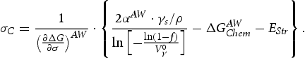
Abstract
The transformation behaviour of retained austenite in steels is known to differ according to chemical composition and other microstructural attributes. Earlier research indicated that austenite in high-carbon steels transforms into martensite only when the applied stress exceeds a critical value, contrary to low-carbon steels where transformation occurs in the early stages of deformation. Although transformation models have been proposed, most are optimised for low-carbon steels. Here, we propose physics-based models applied to high-carbon steels to overcome previous limitations. The models have fewer free parameters (4) compared to previous approaches (6), exhibiting improvements in the numerical and physical interpretation of the austenite transformation process. We envision the use of these models as tools for alloy design, also highlighting their scientific and technological value.
Keywords
Introduction
The presence of retained austenite in steel has implications for its mechanical performance. For example, while retained austenite is reported to enhance the rolling contact fatigue life of bearings [1,2], excessive amounts can compromise its dimensional stability [3]. The opposing effects of retained austenite and its implications for bearing steels have been reviewed by Sidoroff et al. [3].
In a study on the mechanical stability of retained austenite in carburised bearing steels, Bedekar et al. [4] reported the onset of retained austenite transformation into martensite at a critical stress close to the yield point; retained austenite remained stable in the elastic deformation regime. Similar observations were reported in through-hardened steels [5-7]. In contrast, retained austenite in transformation-induced plasticity (TRIP) steels transforms into martensite almost immediately upon loading [8].
The mechanical stability (or kinematic stability) and transformation kinetics of retained austenite have been modelled in several investigations [4,7,9]. These studies employed crystal plasticity finite element models informed by experimental measurements of the transformed amounts of retained austenite. While micromechanical models can simulate the material response in detail, their implementation is complex and requires significant computational resources. Analytical models are simpler to implement, although their dependence on empirical data limits their range of applicability.
Haidemenopoulos et al. [10] developed an analytical model for calculating the critical stress required to transform retained austenite into martensite in a low-carbon steel; the model considers the effect of austenite chemical composition, size, and stress state. The critical stress is calculated to determine the
 temperature, which is an indicator of retained austenite mechanical stability. The application of this model has been demonstrated for low-carbon TRIP [11], quench-and-partition (QP) [12], and Fe-Ni-Co steels [13]. Therefore, it serves as a starting point in the present work.
Models that describe the kinetics of deformation-induced martensite transformation have been developed by previous authors [14-16]. Since these models are fitted to experimental data that are primarily from low-carbon steels, their direct application to high-carbon steels may lead to poor predictions of the transformation progress. This is because the effect of increased carbon concentration on the factors controlling austenite stability is not considered.
For example, the critical driving force to initiate martensite transformation increases with carbon concentration, which leads to the enhanced thermodynamic stability of retained austenite. The effect of carbon concentration also intrinsically affects the influence of austenite morphology [17] and the strength of the martensite matrix [18], where the latter influences the degree of stress–strain partitioning between austenite and martensite [19].
The aim of this work was to develop equations that model the critical stress and progress of deformation-induced martensite transformation in high-carbon steels. The equation developed by Haidemenopoulos et al. [10] was adapted to calculate the critical stress for martensite transformation in high-carbon steels. The critical stress was employed in an equation that calculates the transformed amount of retained austenite with applied stress. Both equations were validated with experimental data from bearing steels. A parametric analysis was conducted to study the limits of the critical stress equation, followed by examples illustrating the application of both equations in alloy design.
Material information
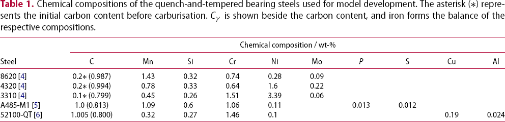
Chemical compositions of the quench-and-tempered bearing steels used for model development. The asterisk (*) represents the initial carbon content before carburisation. is shown beside the carbon content, and iron forms the balance of the respective compositions.
The carbon content in retained austenite
 before mechanical loading is shown beside the nominal carbon content of the respective steels.
 is normally estimated from equations relating the lattice parameter of retained austenite,
 , to the chemical composition. It is acknowledged that the
 could be affected by the effects of auto-tempering and accommodation stress induced by martensitic transformation on
 . However, measurements of the actual
 were not reported in the respective works [4-7], nor the cooling rates to determine possible auto-tempering effects. Given such limitations in the information,
 is estimated from composition-dependent lattice parameter equations.
Since the equations for evaluating
 are different in the respectively noted works,
 is derived based on the following expression to ensure consistency in calculations [6]:
 is the measured austenite lattice parameter in Å and
 is the concentration of the alloying element in wt-%. The value for
 is derived from
 (i.e.
(i.e.
 ) and the concentrations of the other elements follow the bulk composition.
In the work of Foster et al. [6], the original
 for the 52100-QT steel was reported to be 0.593 wt-%C, which is much lower than expected. The
 for a 52100 steel has been reported to be 0.86 wt-%C [20] after undergoing heat treatment similar to the method employed by Foster et al. [6]. Therefore, the
 of 52100-QT steel in Table 1 is taken as 0.8 wt-%C for calculation purposes. It is also noted that the
 calculated for other steels mentioned in this work (including those in Tables 1 and 6) is close to the values quoted in the respective works [4-7].
Description of the critical stress model
Derivation of the critical stress model
Referring to the work of Haidemenopoulos et al. [10], the derivation of the critical stress model is presented in this section. The modifications made to adapt the original model [10] to high-carbon steels are presented in subsequent sections.
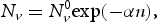
In stress-assisted martensite nucleation, the martensite nucleates at pre-existing sites within the parent austenite grain, which are the same nucleation sites where transformation under quenching occurs [21,22]. The applied stress influences the transformation kinetics by changing the potency distribution of these nucleation sites. This distribution can be described by a model of heterogeneous martensitic nucleation developed by Olson and Cohen [23,24].
The potency of a martensitic nucleation site,
 , is represented by the thickness of the nucleus (in terms of the number of crystal planes) that is derived from the disassociation of existing defects. The critical
 at a given thermodynamic driving force per unit volume is [10]:
 is the nucleus specific interfacial energy (J m−2),
 is the density of atoms in the fault plane (mol m−2),
 is the chemical driving force for martensitic transformation (J mol−1),
 is the elastic strain energy (J mol−1), and
 is the frictional work of interfacial motion (J mol−1).
When an external stress is applied, a mechanical driving force,
 (J mol-1), is added to
 in Equation (2) to give the total driving force as:

 varies with applied stress,
 (in MPa), according to:
 (J mol−1 MPa−1) represents the stress state of the transforming plate [25].
Based on Equation (2), Cohen and Olson [26] derived the number density of operational nucleation sites
 as:
as:
 is the total number density of nucleation sites of all potencies (m−3) and
 is the dimensionless shape factor of the potency distribution [21].
For an austenite particle with volume
 (m3), the fraction of particles that will transform into martensite (
 ) via sites of potency with density
 (m−3) is equal to the probability of finding at least one nucleation site in the particle, assuming the austenite particle transforms into martensite in a single nucleation event [13]. This probability is given as [26]:
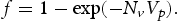
 (in MPa), can be expressed as:
 ,
,
 ,
,
 , and
, and
 ) and six free parameters (
 ,
,
 ,
,
 ,
,
 ,
,
 , and
, and
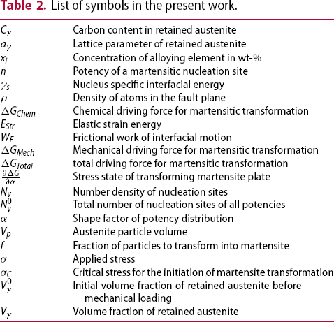
 ). A list of symbols used in the present work and their definitions is shown in Table 2.
List of symbols in the present work.
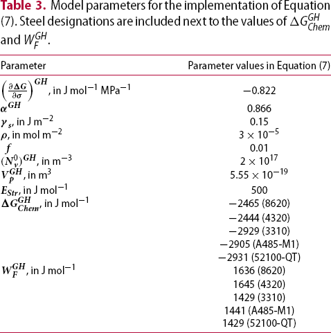
Calculation of parameters in Equation (7)
Equation (7) has been implemented to estimate the
 for the quench-and-tempered steels investigated. Details of the calculation using Equation (7) are presented in this section. For clarity, the parameters calculated using equations in the work of Haidemenopoulos et al. [10] are denoted with the superscript ‘GH’; the latter represents the author's initials (e.g.
 ).
).
According to Haidemenopoulos et al. [10],
 (J mol−1) is calculated using the following linear expression:
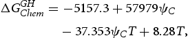
 is the mole fraction of carbon in austenite and
 is the temperature in degrees Celsius.
The parameter
 (in J mol−1 MPa−1) is calculated according to the expression [10]:
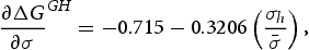
 is −1/3 for uniaxial compression, 1/3 for uniaxial tension and 0 for pure shear.
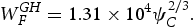
 (in J mol−1) is calculated according to the expression [10]:
Model parameters for the implementation of Equation (7). Steel designations are included next to the values of and .
Modified critical stress model
The modifications made to adapt Equation (7) for calculating the
 of high-carbon quench-and-tempered steels are presented in this section.
In the earlier works of Haidemenopoulos et al. [11,13], the value for
 was estimated to be 2 × 10¹⁷ m−3. This value is derived from the work of Cohen et al. [26,27], which is based on fitting Equations (2) and (5) to the experimental data from Cech and Turnbull's small particle experiments which involved using a Fe-30Ni wt-% steel [28]. However,
 was found to be in the order of 1.5–4 × 10¹⁷ m−3 when fitted to experimental data from TRIP steels [21].
Similarly, the austenite particle volume,
 , is not a constant value since it could be influenced by the type of steel and heat treatment employed. For instance,
 has been reported to be 5.55 × 10⁻¹⁹ m3 for a 4340 steel [10] and 4.18 × 10⁻¹⁸ m3 for a TRIP steel [21]. The latter is based on TEM measurements of austenite particles with a mean radius of R = 1 µm [29], in which a spherical volume has been assumed for simplicity. In another work [30],
 is found to be in the order of 10−20 m3 based on an undeformed austenite particle diameter of 0.35 µm.
These reports show that the determination of
 depends on the measured austenite particle size. While the dispersed austenite particles in the works of Haidemenopoulos et al. [10,21] are assumed to be spherical, this assumption cannot be applied to steels in the current work because the morphology of retained austenite was reported to appear as complex, heterogeneous, and interconnected in a tempered microstructure [4]. The size of retained austenite grains in tempered microstructures is also rarely reported, so any assumptions based on steels of other microstructures could lead to inaccurate calculations of
 .
.
The determination of
 and
and
 is challenging given that they are material-dependent and require experimental measurements that cannot be obtained easily. An easier approach is to consider the product of these parameters
 as equivalent to the initial retained austenite volume fraction before mechanical loading,
 . By multiplying
 (∼ × 1017 m−3) with
 (∼ × 10−18 m3), the product is a dimensionless quantity (∼ × 10−1) with a magnitude that is within the order of typical retained austenite volume fractions.
A similar approach was previously taken by Haidemenopoulos et al. in which the size effect of austenite particles is expressed as a scaled radius
 [13]. While the effects of
 and
and
 are not explicitly considered in the modified equation, the advantage of condensing these effects into the
 term is that
 can be easily measured with conventional experimental methods such as XRD.
The calculation of
 for the quench-and-tempered steels using Equation (8) leads to an inaccurate calculation of
 . This is because Equation (8) is not valid for the composition range of the high-carbon steels investigated. The absence of concentration terms that account for other elements that can affect the driving force (e.g. nickel, manganese) is another limiting aspect for the application of Equation (8) in the present work.
Nowadays, it is convenient to calculate the Gibbs free energy with thermodynamic software.
 is calculated using Thermo-Calc software with the TCFE 8.1 database [31] in this study. For the present calculations, the chemical composition of retained austenite follows the composition of the respective steels in Table 1, where
 after the evaluation of
 from Equation (1). While it is acknowledged that
 can vary locally with different retained austenite grains, especially in carburised specimens, to simplify the calculations the current work assumes that
 is uniform across the microstructure. Since the quench-and-tempered steels were tested at room temperature, a temperature of 20°C was used in the thermodynamic calculations.
 for the quench-and-tempered high-carbon steels, the
 values calculated with Equation (7) were significantly higher than the experimental values (see Table 5). Since
 and
and
 in Equation (7) are the terms that directly vary with chemical composition, the overestimation of
 is likely caused by inaccurate values of
 and
and
 .
.
Model parameters for the implementation of Equation (11).
The measured and calculated for the quench-and-tempered steels.
 /MPa
/MPa MPa
MPaMaterial parameters, measured and calculated for steels with alternative microstructures.


 , Equation (11)
Because martensite transformation occurs via the movement of a glissile interface, the transformation can be suppressed by microstructural features that obstruct the mobility of the interfacial dislocations. The composition dependence of
 arises from the fact that the resistance to dislocation motion was found to vary with solute concentration [32].
The limitations of a composition-based expression for
 (i.e. Equation (10)) are similar to those described for
 earlier. Haidemenopoulos et al. previously expressed
 as a function of carbon and manganese in [11], and nickel in [13]. While these linear expressions might be valid for low-carbon steels or those with simple alloying systems, they are not directly applicable to the present steels. This is because the validity of the
 expressions developed in [11,13] and [10] does not cover the composition of multicomponent high-carbon steels such as those in the present investigation. Attempts have been made to apply the
 expression developed by Ghosh and Olson [32] (which considers multicomponent steel systems) in Equation (7) to calculate
 . However, the differences between the calculated and experimental
 values were significant, possibly due to errors that arise from limiting assumptions in the
 expression developed by Ghosh and Olson [32].
In subsequent calculations using the modified critical stress model, where
 is replaced with
 , it was found that reasonable values of
 can be obtained without including
 in the calculations (see Table 5). It is acknowledged that the exclusion of
 might indicate that the effect of alloying elements in impeding the mobility of the martensitic interface is not considered explicitly in the modified critical stress model.
However, the numerical contribution of
 to the energy balance is likely to be incorporated in the
 term, such that the net difference between
 with
with
 and
and
 results in
 calculations that are close to experimental values. The application of a
 expression that is not valid for high-carbon, quench-and-tempered steels results in incorrect calculations of
 . To the best of the author's knowledge, there is currently no
 expression that is suitable for high-carbon steels with quench and tempered microstructure. The development of such an expression for
 , if at all necessary, is a task for future work.
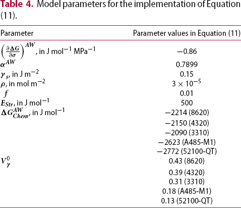
The values for the terms
 ,
,
 ,
,
 , and
, and
 in the modified model are 0.15 J m−2, 3 × 10⁻⁵ mol m−2, 0.01, and 500 J mol−1, respectively [11,24]. If martensite transformation is assumed to initiate on the most favourably oriented nuclei, the value of
 is −0.86 J mol−1 MPa−1 when the stress state is in uniaxial tension [25]. This applies to all the steels in the present work since they were subjected to uniaxial tensile tests.
The shape factor
 is fitted by using the Curve Fitter app in MATLAB 2022a. The procedure involves defining
 and
and
 as the independent variables, whereas the measured
 of the quench-and-tempered steels [4-6] is defined as the dependent variable (under ‘Select Data’ in the app, set
 ,
,
 , and measured
 as the ‘X Data’, ‘Y Data’, and ‘Z Data’, respectively). The shape factor
 is obtained by fitting these variables into the modified critical stress model (under ‘Fit Type’ in the app, select the ‘Custom Equation’ mode and insert Equation (11)), while keeping the values of other parameters (see Table 4) unchanged. This yields a value of 0.7899 (±0.0215) for the shape factor
 .
.
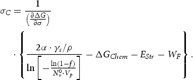
Therefore, the modified critical stress model is expressed as:
 ,
,
 ,
,
 , and
, and
 ) and four free parameters (
 ,
,
 ,
,
 , and
, and
 ). Note that the number of free parameters in Equation (7) has been reduced from six to four in Equation (11) by replacing
 and
and
 with
with
 and removing
 . This shows that the modified model requires fewer free parameters to calculate the critical stress of martensite transformation in high-carbon quench-and-tempered steels.
Description of the austenite volume fraction model
The derivation of a model that calculates the volume fraction of retained austenite,
 , as a function of applied true stress,
 is presented in this section. Martensite transformation occurs when
 . If the steel is mechanically loaded at a constant temperature,
 is assumed to remain constant. The martensitic transformation is solely driven by
 , which is a function of
 . For the steels investigated in this work,
 was observed to decrease with
 when
when
 is greater than
 [4-6].
If the change in the martensite fraction
 for a given increment of
 is proportional to
 , then:
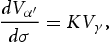
 is a constant.
Since
 , integration of Equation (12) gives:
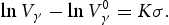
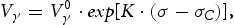
 is greater than
 , the
, the
 when
when
 is set to be equal to
 . The term
 (MPa−1) represents the slope of the function and is fitted by plotting the experimental values of
 versus
 for the linear, decreasing segment of the experimental transformation curves [4-6]. The values of
 for 8620, 4320, 3310, A485-M1, and 52100-QT steels are −4.948 × 10⁻⁴, −5.108 × 10⁻⁴, −5.389 × 10⁻⁴, −7.307 × 10⁻⁴, and −6.09 × 10⁻⁴ MPa−1, respectively. A value of
 = −5.768 × 10⁻⁴ is obtained from the average of the
 values of these steels, and this value is applied in subsequent calculations using Equation (14).
Determination of
 and
and
 from experimental data
The experimental values of
 and
and
 are determined from the retained austenite volume fraction and true stress measured during the uniaxial tensile tests of the steels. These tests were performed using neutron diffraction (for 8620, 4320, 3310, and A485-M1 steels) and synchrotron XRD (for 52100-QT steel). The models were validated with measured
 and
and
 from experimental datasets provided by the respective authors [4,5] for the first group of steels, while the experimental
 and
and
 values for 52100-QT steel were obtained by digitising the results reported in [6].
The authors in [4-6] did not define a procedure for determining
 from the transformation curves. Therefore, the selection of
 was arbitrary and most likely corresponds to the highest value of
 before an apparent decrease in
 was observed. The same approach was adopted to determine
 from the experimental datasets of the steels in the present study.
Results
Calculated
 for steels with quench-and-tempered microstructures
The calculations of
 are performed according to the original and modified critical stress models. Values of the model parameters are described in Tables 3 and 4.
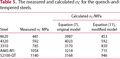
Table 5 shows the experimentally measured and calculated
 for the quench-and-tempered steels as mentioned in Table 1. The
 values calculated using Equation (7) are significantly higher than the measured values for the respective steels, whereas the calculated values from Equation (11) are closer to the measured values. The difference between measured and calculated
 values for the 8620, 4320, and 3310 steels are within ± 45 MPa, whereas those for the A485-M1 and 52100-QT steels are within ± 345 MPa. Despite the differences, Equation (11) performs better than Equation (7) in calculating
 for quench-and-tempered high-carbon steels.
Calculated
 for steels with alternative microstructures
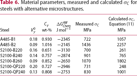
The application of Equation (11) in steels with other microstructures is assessed by calculating the
 for bainitic and quench-and-partitioning (QP) steels. According to Table 6, the steels are labelled according to their respective designations in [7] (for A485 steel) and [6] (for 52100 steel). The heat treatments of these steels are described in [6,7]. The
 is calculated with Equation (11) according to the procedure described in Section 3.3. The
 for the steels is calculated with Equation (1). The concentrations of the other alloying elements are assumed to follow the respective compositions of the A485-M1 and 52100-QT steels in Table 1.
Table 6 shows the measured and calculated
 values for bainitic and QP steels. When comparing the steels subjected to the same type of heat treatment (i.e. A485-B1/B2; 52100-B220/240/260; 52100-QP220/240), the measured and calculated
 values increase when the magnitude of
 is smaller and when
 decreases. Despite the ability of the model to correctly predict the variation of
 with
with
 and
and
 , the differences between the measured and calculated
 values are large — on the order of ±135–800 MPa. Possible reasons are discussed in Section 7.1.
Calculated
 for steels with quench-and-tempered microstructures
Figure 1 shows the variation of
Measured and calculated retained volume fraction (
 with the measured true stress of the quench-and-tempered steels [4-6], where
 is calculated with Equation (14). The region of mechanical stability is indicated by the portion of the curve where
 remains constant. The transition point on the curve represents the onset of martensite transformation when
 . A comparison of the curves shows that the transformation initiates at later stages as
 becomes higher. Based on Figure 1, 52100-QT has the highest
 and, therefore, the most mechanically stable retained austenite among the quench-and-tempered steels. The curves predicted by Equation (14) agree well with the experimental data.
 ) of steels with quench-and-tempered microstructure.
Calculated
 for steels with alternative microstructures
The utility of Equation (14) is assessed by calculating the
Measured and calculated retained austenite volume fraction (
 for the bainitic and QP steels described in Section 6.2. The calculation is performed by setting
 according to the measured
 values of the respective steels in Table 6. The model is also applied to predict the transformation curve for a TRIP steel that was tensile-tested at 293 K [8]. Since the TRIP steel showed immediate retained austenite transformation upon loading,
 is calculated by setting
 as 0 in Equation (14). Based on the transformation curves shown in Figure 2, the
 calculated with Equation (14) show good agreement with the experimental data.
 ) of bainitic, QP and TRIP steels. The transformation curves are shown in separate plots for clarity.
Discussion
Critical stress for retained austenite to martensite transformation
Referring to Table 6, steels subjected to the same type of heat treatment (i.e. A485-B1/B2, 52100-B220/240/260, and 52100-QP220/240) exhibit higher
 values when the magnitude of
 is smaller. The physical meaning of a smaller magnitude of
 , i.e. lower chemical driving force, is that the retained austenite is more resistant towards martensite transformation, which is caused by a higher
 . This indicates a higher retained austenite stability which means that the martensite transformation initiates at a higher
 .
.
The
 is also observed to increase with a lower
 . However, it is challenging to analyse the effect of
 on the calculation of
 separately from chemical composition effects. The A485-M1 and 52100-QT steels are considered as an example. Although both steels have very similar
 (see Table 1), the magnitude of the
 for 52100-QT is 149 J mol−1 higher than that of A485-M1 steel, presumably due to the effect of other alloying elements on the chemical driving force. If the critical stress is considered only on the basis of chemical composition via the chemical driving force, then the
 of 52100-QT steel is expected to be lower than that of A485-M1 steel because of lower retained austenite stability.
However, the measured
 of 52100-QT (1140 MPa) is higher than that of A485-M1 (1058 MPa). This is most likely because the 52100-QT steel has a lower
 than the A485-M1 steel, which corresponds to a higher amount of martensite in the microstructure before the steel was mechanically loaded.
According to Xiong et al. [17], the martensite plates, which have a higher yield stress than austenite, could obstruct the retained austenite grains from transforming into martensite. This occurs because the martensite matrix surrounding the grains must deform to contain the volume expansion caused by martensitic transformation [17]. They also proposed that the hydrostatic pressure induced by the residual stress generated in the microstructure could hinder martensite transformation, which is accompanied by volume expansion.
Since
 replaces the product
 in the critical stress model, the term
 collectively represents the number density of martensitic nucleation sites and austenite particle volume. The physical meaning of this representation is that a lower
 indicates lesser martensitic nucleation sites so that the martensite transformation is triggered and detected at a higher
 .
.
These reasons could explain why 52100-QT has a higher
 than A485-M1 because of a lower
 , an effect that is reflected by the modified critical stress model.
In Table 6, major differences are observed between the measured and calculated
 values for bainitic and QP steels. Bainite is reported to dominate the bainitic and QP microstructures of the corresponding A485 [33] and 52100 [6] steels. Therefore, the large differences in
 are most likely a result of the influence of bainite on the load partitioning behaviour; thus, its subsequent effect on austenite stability is not considered in the modified critical model.
When a composite microstructure containing phases of variable properties is stressed, the soft phase that is more ductile is the first to deform plastically. The deformation is followed by work hardening. The load will be eventually transferred to the harder phase [34]. Therefore, in a microstructure containing phases of varying strengths, the critical transformation stress of retained austenite also depends on the mechanical response of the surrounding phases when deformation is applied.
Referring to a study on austenite stability and strain evolution in TRIP-assisted steels as an example [35], the matrix composed of ferrite and bainitic ferrite was found to have the lowest load-bearing capacity, followed by austenite and martensite. The authors also reported that the transformation of austenite into martensite in the steel with more bainitic ferrite occurred at later stages of the deformation due to delayed work-hardening of the matrix microstructure [35]. These observations can be related to the relative strengths of the phases present in the microstructure [36].
According to the work of Foster et al. [6], the
 increases with
 and the amount of bainitic ferrite in the steels with bainitic (i.e. 52100-B) and QP (i.e. 52100-QP) microstructures. However, these steels have a lower
 than the 52100-QT steel, which has a tempered martensite microstructure. The varying austenite stabilising effects conferred by these different matrices were attributed to the presence of nano-carbides and local straining of the bainitic ferrite surrounding the austenite grains [6]. These observations point to the major effect of the surrounding matrix on austenite stability.
Currently, the modified critical stress model does not consider explicitly the austenite stabilising effect of the surrounding matrix microstructure. Since the model parameters are fitted based on the composition and microstructure of tempered martensitic steels, the
 calculated with the modified model is expected to differ significantly from the measured
 of steels with other microstructures. The incorporation of the austenite stabilising effects by the surrounding matrix in relation to some of the aforementioned factors is considered for future work on the critical stress model.
Kinetics of deformation-induced martensite transformation
Based on the measured and predicted
 as shown in Figures 1 and 2, the application of Equation (14) appears to work for all steel microstructures in the current investigation. However, the model may underestimate (e.g. for A485-B1 steel in Figure 2) or overestimate (e.g. for 52100-QP220 steel in Figure 2)
 during retained austenite transformation. This is because the average
 value as mentioned in Section 4, i.e.
 = −5.768 × 10⁻⁴, is applied in all calculations, which may be slightly different from the
 value obtained from each dataset.
Nonetheless, the model predictions are in good agreement with measured values, demonstrating that the model can predict the retained austenite fraction for stress-induced martensite transformations in the investigated steels regardless of whether the steel exhibits a delayed transformation of retained austenite.
Parametric analysis of the critical stress model
To determine the constraints of the critical stress model, the influences of
 and
and
 on
on
 are examined. A parametric analysis of Equation (11) is conducted by calculating the
 of 8620 steel (see Table 1) across a range of
 and
and
 values while keeping the other parameters constant.
Since
The change in critical stress
 changes with chemical composition, the effect of chemical composition is assessed by calculating
 across a range of concentrations for the austenite stabilisers (carbon, manganese, and nickel) at a constant temperature of 20°C and
 of 0.43. Based on Figure 3(a), the
 increases with higher concentrations of carbon, manganese, and nickel. The austenite stabilising effect of these elements raises the free energy required to initiate martensite transformation. Since
 to initiate martensite transformation, a higher
 is needed, which is indicated by a higher
 . Furthermore, the rate of increase in
 per wt-% alloying element is highest for carbon, followed by manganese and then nickel. This observation agrees with the reported austenite stabilising potencies of these elements [37], where carbon is known to be the strongest austenite stabiliser, followed by manganese and nickel.
 as a function of (a) solute concentration; (b) temperature; (c)
 .
.
The effect of temperature on
 is studied by calculating
 at −60°C–160°C, according to the chemical composition of 8620 steel and a
 of 0.43. The selected temperature range is based on standard service temperatures for bearings [38]. The martensite transformation is less likely to occur at elevated temperatures because there is less undercooling available to provide the required thermodynamic driving force through
 . Thus,
 increases with temperature (as shown in Figure 3(b)) because a higher
 is needed to supplement the driving force for martensite transformation.
This observation agrees with the experimental findings of Neu and Sehitoglu [39]. By performing uniaxial tensile tests on carburised 4320 steel across a temperature range of −60°C–50°C, the authors reported decreasing transformation amounts with higher testing temperatures and speculated that little stress-induced retained austenite transformation occurs above 60°C [39].
The experimental findings of Kulin et al. [40] also demonstrated that stress-induced transformation decreases as the testing temperature increases progressively above the
 temperature of a 0.5C-20Ni (wt-%) steel (assumed to be −37°C). They reported that martensite transformation was barely observed at 0°C and non-existent at 20°C, showing that the stress-induced transformation occurred within a narrow range between the
 temperature and approximately 40°C above the
 . Based on the
 equation developed by Bohemen [41], the
 temperature of the 8620 steel is calculated to be approximately 136°C. Thus, it could be implied that minimal or no stress-induced transformation would occur in 8620 steel at testing temperatures higher than 136°C.
The variation of
 with
with
 is evaluated by calculating the
 of 8620 steel at a temperature of 20°C and setting
 to 0.8, 0.9, and 1 wt-%C, respectively. The concentrations of other alloying elements follow that of 8620 steel in Table 1. According to Figure 3(c), the
 increases with
 at a constant
 . When
 is constant, the
 decreases with increasing
 . This trend is consistent with the measured
 of the quench-and-tempered steels (Table 5) with respect to their
 (Table 4), where 8620 steel has the lowest measured
 of 441 MPa but the highest
 of 0.43. In Table 6, steels subjected to the same type of heat treatment also showed higher
 with lower
 . The observation that a higher retained austenite fraction leads to lower critical stress for martensite transformation agrees with the findings of Alley and Neu [9]; the authors described the variation of
 with
with
 through an empirical equation.
Strictly speaking, the relationship between
 and
and
 is linked to the chemical composition and heat treatment of the steel. Considering the 52100 bainitic steels in Table 6 (B220/240/260) as an example, the increasing bainitic treatment temperatures result in higher amounts of austenite decomposing into bainite [6], as the remaining austenite becomes enriched with carbon due to carbon partitioning [34]. This leads to a lower
 and higher
 , thus increasing the stability of the austenite as indicated by a higher
 . Zhou et al. [42] reported high retained austenite mechanical stability during tensile testing of a medium-manganese steel with low
 that contained a high solute concentration and small grain size, which is a consequence of heat treatment.
Despite the good agreement between experimental trends and
 values predicted by Equation (11), the model has its limitations. The main constraint of the model is the range of chemical composition and
 values that were used to develop the model parameters. Consequently, the model predicts negative
 values in certain conditions: below 0.8 wt-%C (Figure 3(a)); at temperatures below −60°C (Figure 3(b)); above
 when
when
 wt-%C; and above
 when
when
 wt-%C (Figure 3(c)).
Equation (11) predicts a negative
 value when
 is greater in magnitude than the energy barrier to martensite transformation, which is defined in the terms
 and
and
 . This could imply that the delayed deformation-induced transformation of retained austenite into martensite does not occur or occurs shortly after mechanical loading. The latter scenario applies to low-carbon TRIP steels [8]; in this case, the critical stress model of Haidemenopoulos et al. [11] might provide better predictions of
 .
.
Another reason for the prediction of a negative
 is because the same value of
 (0.7899) is applied in all calculations. The value of
 was previously reported to be 0.866 by Haidemenopoulos et al. [10,11]. However, Olson et al. [27] reported a value of
 , which they obtained by best-fitting Equations (2) and (5). In the process of fitting
 for the quench-and-tempered steels, it was found that
 is sensitive to carbon content. A lower
 value results in reasonable predictions of
 when
when
 is lower than the current threshold of 0.8 wt-%C (see Figure 3(a)).
This observation agrees with recent work by Haidemenopoulos et al. [21] and Polatidis et al. [30] on low-carbon TRIP steels, where a value of 0.1 was used for the shape factor α. Haidemenopoulos et al. [21] reported that the value of
 should be lower for steels with retained austenite that is less stable. Referring to Equation (5), a low value of
 results in high
 , which implies a higher density of potent martensitic nucleation sites.
 is dependent on the potency of martensitic nucleation site
 , which explains why it is appropriate to use a low
 value to predict
 for retained austenite grains with low stability, such as those with low-carbon content. Inversely, the value of
 is expected to be higher when predicting
 for retained austenite grains with higher stability, as is the case with the high-carbon steels in the present investigation.
The utility of Equation (11) can be extended by assessing the mechanical stability of the retained austenite in high-carbon steels in other stress states. For example, retained austenite in a case-carburised steel has been reported to transform into martensite under rolling contact fatigue (RCF) conditions [43]. The
 parameter in Equation (11) should be modified accordingly when the stress state is different.
The parametric analysis of Equation (11) showed that
 increases with higher austenite stabiliser (carbon, manganese, nickel) concentrations, higher temperatures, and lower
 . While the effects of these parameters on
 have been assessed separately, they are interrelated in practice and should be considered collectively when the model is implemented. The analysis also identified
 as a limiting factor for the application of this model, as it is expected to change with other steel compositions and
 . Despite the model constraints as imposed by the composition and experimental conditions of the quench-and-tempered steels, this model can be extended to other steels by deriving the relevant material parameters following the procedures outlined in Section 3.
Model applications
Potential applications for the critical stress and austenite volume fraction models are explored in this section. Previous research has indicated that higher amounts of retained austenite increase the RCF life of bearings [1,2]. On the contrary, Morris and Sadeghi [43] have reported that higher amounts of retained austenite do not automatically improve the RCF life of bearings; the underlying reason is that the high stability of retained austenite restricts its transformation into martensite when subjected to RCF stresses. They found that the benefits of retained austenite to the improvement of RCF life, regardless of its amount, are realised only when its stability is below a threshold that allows martensite transformation during deformation.
Since
 can be used as an indicator of retained austenite mechanical stability, the following examples highlight the implementation of Equations (11) and (14) in selecting chemical compositions and processing parameters for alloy design.
The first example explores different alloy compositions for defined ranges of
(a) Required manganese and nickel concentrations for a range of critical stresses at a deformation temperature of 20°C and
 . By setting a temperature of 20°C and
 of 0.43,
 is calculated within a composition range of 0–3 wt-%Mn and 0–3 wt-%Ni, in steps of 0.1 wt-% Mn/Ni. The concentrations of carbon and other alloying elements follow that of 8620 steel (see Table 1). Figure 4(a) shows the required manganese-nickel combinations in austenite as
 is varied, in which higher concentrations of manganese and nickel increase
 .
.
 of 0.43; (b) change in retained austenite volume fraction
 with applied stress for selected compositions.
To illustrate how variation in the CALPHAD calculations, e.g. by Thermodynamic database accuracy, could affect the model calculations, a sensitivity analysis is conducted, via minor changes in the chemical composition to estimate model variations. When the manganese concentration is set as 1.4 wt% in 8620, the calculated
 for nickel concentrations of 0, 0.2, 0.4, 0.6, 0.8, 1, 1.2, and 1.4 wt-% are 407, 445, 482, 519, 556, 594, 631, and 669 MPa, respectively. When the nickel concentration is set as 1.4 wt-%, the calculated
 for manganese concentrations of 0, 0.2, 0.4, 0.6, 0.8, 1, 1.2, and 1.4 wt-% are 311, 355, 403, 453, 505, 558, 612, and 669 MPa, respectively. The results demonstrate a model sensitivity of ∼200–220 MPa/wt% for
 , indicating relatively low sensitivity to possible changes in the CALPHAD predictions, given the narrow range in compositional differences in high-carbon steels (<1–2 wt%, Table 1) and the accuracy in the predicted results in Table 5 for several steels. Further assessment on the accuracy of the CALPHAD calculations is beyond the scope of the present work.
In bearing applications, the chemical composition should be selected to ensure that retained austenite remains stable at the applied loads during service. Figure 4(a) can be used as a guide to select suitable alloy compositions for a defined range of
 . Since the price of manganese is lower than nickel [44], using a high manganese-low nickel combination may make it possible to manufacture bearings at significantly lower prices than those alloys in current use.
Figure 4(b) shows the stress-induced transformation progress of retained austenite for various manganese concentrations when the deformation temperature and nickel concentration are fixed at 20°C and 0.1 wt-%, respectively. As the manganese concentration increases, martensite transformation initiates at higher
 values and a higher amount of retained austenite is left when the stress is removed. Figure 4(b) can be used to inform the selection of manganese-nickel combinations that optimise martensite transformation (i.e. the ‘TRIP effect’) and to control the amount of retained austenite; this is useful in metal forming operations.
The second example explores different alloy compositions for a defined range of
(a) Required manganese and nickel concentrations for deformation temperatures between −50°C and 80°C with
 at various deformation temperatures. Setting
 as 0.43 and following the composition of 8620 steel, the calculation is performed within a temperature range of −50°C–80°C in steps of 10°C and 0.05 wt-% Mn/Ni. The calculation is also constrained to compositions that result in
 between 400 and 500 MPa (noting that the measured
 of 8620 steel is 441 MPa). According to Figure 5(a), the concentrations of manganese and nickel required to achieve
 within the target range increase with lower deformation temperatures. Since retained austenite transforms more easily into martensite at low temperatures due to greater undercooling, a higher concentration of austenite stabilisers is needed to maintain austenite stability.
 values within a range of 400–500 MPa; (b) change in retained austenite volume fraction
 with applied stress for a composition of 1.4Mn-0.3Ni (wt-%) within a temperature range of −40°C to 120°C.
It was found that
 exceeds 500 MPa when the deformation temperature is above 80°C. Figure 5(b) shows the changes in
 with
with
 at different temperatures. The composition is set as 0.3Mn-1.4Ni (wt-%) because this combination is closest to that of 8620 steel (see Table 1). As temperature increases, martensite transformation occurs at higher critical stresses with lesser retained austenite remaining after the stress is removed; no transformation occurs at 120°C. Considering the service temperature range for most rolling-element bearings (i.e. ranging from −50°C up to the order of 120–150°C) [38], the dimensional stability of bearings is critical as fluctuations in service temperature can induced retained austenite decomposition. Therefore, the information from the calculations shown in Figure 5 can aid the design of bearing compositions that optimise retained austenite stability against the transformation induced by temperature fluctuations, which is crucial for bearings operating in extreme environments.
The examples have shown the utility of the models in predicting the parameters for optimal austenite stability in bearing applications once a target stress and/or strain are defined. However, the influence of heat treatments and manufacturing processes should also be considered, as the models do not explicitly account for these factors. For instance, while it is known that manganese can promote austenite stability as well as nickel but with higher cost-effectiveness, excessive amounts of manganese can cause surface and internal oxidation in carburised steels [45]. Therefore, these models should be implemented together with other manufacturing considerations to inform the design process of new bearings.
Conclusions
In this work, models for predicting the critical stress and progress of deformation-induced martensite transformation in high-carbon steels have been developed. The critical stress model (Equation (11)) was developed to overcome the limitations of existing models when predicting
 in high-carbon quench and tempered steels, which exhibit delayed retained austenite transformation under applied stress. Compared to Equation (7), i.e. the model of Haidemenopoulos et al. [10], Equation (11) requires fewer free parameters (i.e. reduced from six to four), providing better physical and numerical interpretations in the parameter selection and reduction to study TRIP in high-carbon steels. Calculations of
 with Equation (11) are in good agreement with measured values from the investigated quench-and-tempered steels.
Equation (11) considers the influence of chemical composition, deformation temperature, and initially retained austenite fraction on
 . Higher austenite stabiliser concentrations in the composition or higher deformation temperatures result in austenite that is more stable against transformation; these effects are represented by a smaller magnitude of
 . A lower
 indicates fewer martensitic nucleation sites, which means that the martensite transformation under applied stress occurs at a higher
 .
.
Since the critical stress model was developed based on steels with microstructures that consist primarily of tempered martensite and retained austenite, the accuracy of the model predictions diminishes when applied to steels with other microstructures. In contrast, the model for calculating the transformed amounts of retained austenite under applied stress (Equation (14)) was found to perform well when applied to steels that exhibit (i.e. high-carbon steels) or do not exhibit (i.e. low-carbon steels) the delayed retained austenite transformation phenomenon.
A parametric analysis of Equation (11) showed that
 increases with higher austenite stabiliser concentrations, higher deformation temperatures, and lower
 . Besides identifying the limiting conditions of the model, the analysis highlighted the sensitivity of the shape factor
 to material parameters, notably
 . Potential model applications have been explored. It is anticipated that these models can be used to aid the design of new alloy compositions for bearings with optimal retained austenite stability and cost-effectiveness.
Footnotes
Acknowledgements
Adriel Wong gratefully acknowledges the financial support provided by The Timken Company for this work as part of a PhD project. Enrique Galindo-Nava acknowledges funding from RAEng in the form of a research fellowship.
Disclosure statement
No potential conflict of interest was reported by the authors.