Sage Journals: Discover world-class research

Abstract

Objective: Although the debate on whether mental disorders are categorical or dimensional is critical for researchers and practitioners, past findings of taxometric studies of depression have been somewhat contradictory and difficult to reconcile. One reason for the disagreement was that most researchers relied only on selected samples (students, clinical patients, or screened community samples). The present study investigated whether the latent structure of depression is categorical or dimensional using an unselected general community sample.

Method: To determine whether the latent structure of depression assessed by the Center for Epidemiologic Studies Depression Scale is categorical or dimensional, taxometric procedures were carried out on a Japanese general population-based sample of 20 987 individuals selected using a cluster sampling procedure.

Results: Both the means above and below a sliding cut (MAMBAC) and the maximum eigenvalue (MAXEIG) procedures, using indicators drawn from the Center for Epidemiologic Studies Depression scale yielded results that the latent structure of depression is dimensional.

Conclusions: The dimensional structure of depression should be considered when classifying individual differences and selecting suitable research designs.

Keywords

classification nosology taxometry validation

Are there any boundaries that separate mental disorders from normal conditions? Current diagnostic systems in psychiatry, such as the DSM and ICD, have based a categorical classification system that divides mental disorders into types based on criterion sets with defining features, regardless of whether there are any boundaries between normal and abnormal conditions [1, 2]. Although it is pragmatically useful to draw a line somewhere and make a categorical diagnosis, many researchers have argued that the dimensional classification in the diagnostic systems is a viable alternative [3]. The debate of whether mental disorders are categorical or dimensional (i.e. the continuity controversy) is a research agenda for the ongoing revision of the DSM [4, 5].

Flett et al. described four approaches that have been applied to the investigation of the continuity controversy with regard to depression, namely, the phenomenological, typological, aetiological, and psychometric approaches, and concluded that most of the existing research supports the dimensional model of depression [6]. This conclusion, however, was limited by serious methodological and statistical shortcomings. Recognizing the limitation of existing evidence, Flett et al. called for studies utilizing sophisticated statistical techniques [6], called taxometric procedures, that examine the latent structure of a given construct such as depression [7–9]. In response to this suggestion, a number of investigators have performed taxometric investigations of various mental disorders [10, 11].

In the literature on depression, there are several taxometric investigations. Whereas a few taxometric investigations focus on subtypes of depression, such as hopelessness [12], endogenous [13], or melancholia [14], others focus on general depression (Table 1). To the best of our knowledge, there are 13 taxometric investigations of general depression using various sampling methods, assessments of depression, and statistical analyses (Table 1). Four studies have used students [15–18], five have used clinical samples [19–22], and two have used screened community samples [23, 24]. These differences may introduce disconcerting conclusions about the latent structure.

Table 1.

Summary of previous taxometric investigations of depression

Study	Sample	Assessment	Simulation	n	Results
Baldwin and Shean (2006) [15]	Students	Self-report	Yes	392	Dim
Beach and Amir (2003) [16]	Students	Self-report	No	3936	Cat
Okumura et al. (2009) [18]	Students	Self-report	Yes	2187	Dim
Ruscio and Ruscio (2002) [17]	Students	Self-report	Yes	2260	Dim
Franklin et al. (2002) [19]	Patients	Self-report	No	2000	Dim
Ruscio and Ruscio (2000, Study 1) [20]	Patients	Self-report	No	996	Dim
Ruscio and Ruscio (2000, Study 2) [20]	Patients	Self-report	No	13 707	Dim
Ruscio et al. (2007) [21]	Patients	Interview	Yes	1800	Cat
Slade (2007) [22]	Patients	Interview, Self-report	Yes	960	Dim
Prisciandaro and Roberts (2005) [23]	Screened community	Interview	Yes	4577	Dim
Slade and Andrews (2005) [24]	Screened community	Interview, Self-report	Yes	1933	Dim
Hankin et al. (2005) [25]	Unselected youth	Interview	Yes	845	Dim
Solomon et al. (2006) [26]	Unselected students	Interview, Self-report	No	1500	Cat

Cat, categorical; Dim, dimensional; Simulation, whether or not the bootstrap simulation method developed by Ruscio et al. [27] was used.

As shown in Table 1, most of the previous studies have relied on samples from selected populations, which may cause methodological problems. These sampling procedures lead to an artificial truncation of the depressive symptom severity that can distort results by violating the assumption of conditional independence needed to obtain unbiased estimates [28], and such selection bias can complicate formal inferences about the latent structure [29]. In studies using students, a focus only on students attending classes introduces systematic sampling bias. That is, the data collected in classes are limited to high-functioning (i.e. low in depression) students, because low-functioning (i.e. high in depression) students may be absent [25]. Moreover, focusing only on clinical patients or screened community samples introduces institutional bias, because high-functioning individuals may not be included in these studies [23]. Therefore it is important to use unselected samples with a full range of depression severity.

As far as we know, there are two studies using unselected samples [25, 26]. Hankin et al. used taxometric procedures on an unselected youth sample aged 9–17 years old, and found evidence that the latent structure of depression was dimensional [25]. Still, Solomon et al. noted that the limitation of their study was the assessment of depressive symptoms, which involved reference to the presence of depression at any time in the preceding year [26]. Still, Solomon et al. noted that the limitation of the Hankin et al. study was the assessment of depressive symptoms, which involved reference to the presence of depression at any time in the preceeding year [26]. Previous findings using unselected samples, however, focus only on the structure of depression among a relatively young population. It will therefore be important for taxometric studies of depression to sample unselected community populations to aid generalizability of the previous findings. The present study attempted to solve this problem by conducting a secondary analysis of the Japanese national survey of physical and mental well-being [30]. The main research question investigated in this paper is whether depression assessed using the Japanese version [31] of the Center for Epidemiologic Studies Depression scale (CES-D) [32] is categorical or dimensional.

Method

Data source

Participants were community volunteers who were selected as part of the Japanese national survey of physical and mental well-being [30]. The survey was conducted in June 2000 by the Japanese Ministry of Health and Welfare (the present Ministry of Health, Labour and Welfare). A total of 32 022 people who were ≥ 12 years old were randomly selected from the Japanese population using a cluster sampling procedure. Three hundred clusters were randomly selected from geographical districts. Survey teams visited all the members aged ≥ 12 years old of households in each cluster and asked them to complete the questionnaire. Beginning with the complete data set, we retained a subset of cases for the present investigation according to two conservative criteria. First, cases flagged in the database because of suspect response validity (e.g. those who answered ‘Rarely or none of the time’ for all items regardless of the valence of items) were removed from the sample. Second, cases with missing data on the CES-D, sex and age were also removed from the data set. A final sample of 20 987 cases satisfied the two inclusion criteria. The final sample was 51% female (n = 10 793) and included a broad range of ages (mean = 42.05 years, SD = 18.03, range = 12–97 years).

Measure

To measure depression symptoms, we used the Japanese version [31] of the CES-D [32], which consists of 20 items chosen to reflect the various aspects of depression. Respondents report the frequency of occurrence with regard to each item during the preceding week on the following 4-point scale: 0 = rarely or none of the time, less than 1 day), 1 = some or a little of the time, 1–2 days, 2 = occasionally or a moderate amount of time, 3–4 days, and 3 = most or all of the time, 5–7 days. The summed score of the 20 items can range from 0 to 60, with higher scores indicating more severe depressive symptoms. Four of the CES-D items are symptom positive and are reverse scored. Researchers most often use a CES-D cut-off score of 16 to identify respondents with clinically relevant levels of depression in a community sample [33].

Data analyses

Indicators drawn from the CES-D were subjected to a series of taxometric procedures developed by Meehl and Yonce, and Waller and Meehl for the purpose of examining the latent structure of depression [7, 9]. Taxometric procedures explore the relations among a set of manifest variables in order to determine whether their underlying structure is categorical or dimensional. The latent structure of depression was evaluated using two mathematically distinct taxometric procedures: means above and below a sliding cut (MAMBAC) [7], and maximum eigenvalue (MAXEIG) [9]. The MAMBAC and MAXEIG were performed with two non-redundant sets of indicators drawn from the CES-D. Furthermore, the bootstrap simulation method developed by Ruscio et al. [27] was used to create 100 simulated taxonic and 100 simulated dimensional data sets with skews and correlations that were similar to those of the indicators drawn from the CES-D. The Ruscio et al. method helps researchers evaluate the suitability of research data for taxometric procedures, and facilitate the interpretation of taxometric results. To interpret taxometric curves, we computed the values of the comparison curve fit index (CCFI) [27]. This index assesses the degree to which an averaged curve, obtained through analysis of research data, resembles curves in the sampling distributions of simulated dimensional and taxonic data set. A CCFI value near 0.50 can indicate an equally good or equally poor fit for the two structures; a CCFI value close to 0 and 1 can indicate a dimensional and taxonic structure, respectively. We performed taxometric procedures using the Ruscio taxometric software program for R [34, 35].

Because we retained a subset of cases (n = 20 987) according to two conservative criteria (i.e. removing cases with suspected response validity, and with missing data on the CES-D, sex and age), it is possible that these criteria might have biased the results. In addition, the inclusion of children as young as 12 years old in the sample could potentially bias the sample in some way. We therefore carried out sensitivity analyses. First, we created the following four datasets: (i) removal of subjects with suspected response validity, and with missing data on the CES-D (n = 21 094); (ii) removal of subjects with suspected response validity, and with missing data on the CES-D, sex and age, and inclusion of subjects aged ≥ 18 (n = 19 151); (iii) removal of subjects with suspected response validity, and with missing data on the CES-D, and inclusion of subjects aged ≥ 18 (n = 19 258); and (iv) imputing missing data on the CES-D using a multiple imputation method [36] (n = 32 022). Second, on each dataset we performed the MAMBAC and MAXEIG following the aforementioned procedures.

Results

Selection and construction of indicator

In taxometric procedures, two indicator sets were created from the CES-D items (Table 2). The first indicators (i.e. paired-item) were formed by summing the CES-D items in pairs. Of the 20 CES-D items, 10 were selected on the basis of two criteria. First, we computed the item-total correlations. Because the total score on the CES-D was expected to differentiate normal conditions from clinically relevant levels of depression, items that had high correlations with the total score were identified as valid indicators. Second, to avoid redundancy among indicators, we paired these items in a manner that yielded higher correlations between paired items than between unpaired ones. The final 10 items yielded five paired indicators, each ranging in value from 0 to 6. The second indicator set (i.e. factor analysis) was constructed based on the results of the factor analysis [37]. Sheehan et al. investigated the measurement structure of the CES-D and identified the following four factors: Somatic/Vegetative, Depressed Affect, Positive Affect composite, and Interpersonal Relations [37]. We followed the factor structure, and summed the CES-D items corresponding to the factors.

Table 2.

CES-D items selected for use in taxometric procedures

Item	Wording
1^†	Bothered
2^†	Poor appetite
3^‡	Blues
4^§	Felt as good as others (reverse scored)
5^§,††	Hard to concentrate
6^‡,††	Depressed
7^†,††	Everything an effort
8^§	Hopeful (reverse scored)
9^¶,††	Failure
10^¶,††	Fearful
11^†	Restless sleep
12^§	Happy (reverse scored)
13^†	Talked less
14^‡,††	Lonely
15^¶,††	People unfriendly
16^¶,††	Enjoyed life (reverse scored)
17^‡	Crying spells
18^‡,††	Sad
19^¶,††	People disliked me
20^†,††	Could not get going

CES-D, Center for Epidemiologic Studies Depression scale. ^†Items combined into the Somatic/Vegetative composite. ^‡Items combined into the Depressed Affect composite. ^§Items combined into the Positive Affect composite. ^¶Items combined into the Interpersonal Relations composite. ^††Used in paired-item indicators; pairs consist of items 6 and 7, 14 and 18, 5 and 20, 9 and 10, and 15 and 19.

We computed the standardized mean difference and within-class correlations in order to determine whether the chosen indicators exhibited sufficient validity for taxometric procedures. The sample was divided into two putative classes, separating subjects with total CES-D scores of 0–15 (n = 14 249) from those with total scores of ≥ 16 (n = 6738). We then estimated the validity with which each indicator distinguished the putative classes by calculating the mean and standard deviation of each indicator within each class and the standardized mean difference of each indicator as the measure of separation (Table 3). Eight of the nine indicators achieved a validity greater than the conventional threshold of d ≥ 1.25 [38]. Finally, we computed within-class correlations. Among the paired-item indicators, within-class correlations averaged 0.24, and among the factor analysis indicators, within-class correlations averaged 0.12, which was well within the tolerance limits of taxometric procedures [38].

Table 3.

Summary statistics and validity estimates

Indicator set	Skewness	Kurtosis	MD + Mean	MD + SD	MD − Mean	MD − SD	Valid (d)
Paired item
Items 6 and 7	1.07	0.57	2.95	1.55	0.76	0.97	1.85
Items 14 and 18	2.06	4.37	1.64	1.50	0.24	0.58	1.44
Items 5 and 20	1.41	1.79	2.24	1.49	0.53	0.84	1.57
Items 9 and 10	1.60	2.56	1.95	1.50	0.47	0.75	1.41
Items 15 and 19	2.61	7.75	1.23	1.39	0.13	0.45	1.27

Factor analysis
Depressed affect	1.79	3.60	4.40	2.75	0.69	1.04	2.09
Positive affect	−0.15	−0.75	7.41	2.30	5.59	3.32	0.60
Somatic/vegetative	1.24	1.63	7.88	3.52	2.06	1.95	2.27
Interpersonal relation	1.93	4.43	3.18	2.35	0.61	0.93	1.68

MD+, total CES-D scores ≥ 16; MD−, total CES-D scores 0–15; Valid (d), Cohen's standardized mean difference between MD+ and MD−.

MAMBAC

MAMBAC procedures were performed on each input/output configuration of variables for each indicator set. Summed input indicators were created by removing one indicator from a given set to serve as the output, and by summing the remaining indicators from that set to serve as the input. The panels of individual curves for MAMBAC and MAXEIG, and of the averaged curves for MAXEIG, using 25, 75, and 100 windows, have been omitted due to space constraints. They are available, on request, from the first author. The averaged MAMBAC curves for each indicator set are shown in the first column of Figure 1, and the averaged MAMBAC curves from the simulated taxonic and dimensional data for each indicator set are portrayed in the second and third columns, respectively. As can be observed in Figure 1, each averaged MAMBAC curve resembled the curves from the simulated dimensional rather than taxonic data, although the averaged MAMBAC curves produced by simulated taxonic and dimensional data appeared somewhat ambiguous. Additionally, we computed the values of the comparison curve fit index (CCFI). The values of the CCFI in the present data set were 0.37 and 0.26, respectively (Table 4).

Figure 1.

Means above and below a sliding cut (MAMBAC) and maximum eigenvalue (MAXEIG) curves of paired-item and factor analysis indicator sets. In each row, the left graph represents the averaged results for the research data; the middle graph, averaged results for 100 sample simulated taxonic comparison data; and the right graph, averaged results for 100 sample simulated dimensional comparison data

Table 4.

Comparison curve fit indices

		MAXEIG^†
Indicator set	MAMBAC	25	50	75	100
Paired-item	0.37	0.28	0.30	0.30	0.28
Factor analysis	0.26	0.20	0.26	0.26	0.31

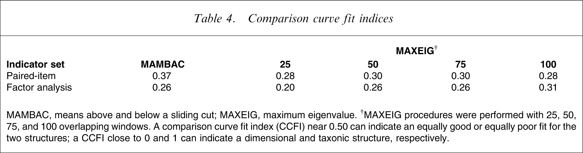
MAMBAC, means above and below a sliding cut; MAXEIG, maximum eigenvalue. ^†MAXEIG procedures were performed with 25, 50, 75, and 100 overlapping windows. A comparison curve fit index (CCFI) near 0.50 can indicate an equally good or equally poor fit for the two structures; a CCFI close to 0 and 1 can indicate a dimensional and taxonic structure, respectively.

MAXEIG

MAXEIG procedures were performed using each indicator as the input and all the other indicators as the output. MAXEIG procedures were repeated with 25, 50, 75, and 100 overlapping windows to implement inchworm consistency test. As can be observed in Figure 1, each averaged MAXEIG curve resembled the curves from the simulated dimensional rather than taxonic data. Additionally, each CCFI ranged from 0.20 to 0.31, with a mean of 0.27.

Sensitivity analyses

We carried out sensitivity analyses to investigate whether the main results were consistent with those obtained with alternative inclusion criteria. On the four datasets, we performed the MAMBAC and MAXEIG procedures. The values of the CCFI on the four datasets ranged from 0.18 to 0.44, with a mean of 0.32. The panels of individual and averaged curves for MAMBAC and MAXEIG, and the values of the CCFI, have been omitted due to space constraints. They are available, on request, from the first author.

Discussion

To determine whether the latent structure of depression is categorical or dimensional, we carried out taxometric procedures on a general population-based sample of >20 000 individuals selected using a cluster sampling procedure. Both the MAMBAC and MAXEIG procedures using indicators drawn from the CES-D yielded results that the latent structure of depression is dimensional. The results of the current study replicate and extend the findings of earlier taxometric procedures of depression (Table 1). Past findings of taxometric studies of depression have been somewhat contradictory and difficult to reconcile. One reason for the disagreement was that most researchers relied only on selected samples (students, clinical patients, or screened community samples). By implementing taxometric procedures in a sample that includes individuals with a wide range of depression severity, the current study extends the conclusion of dimensionality in depression from selected samples to samples in the unselected general community.

Implications of the present study

These dimensional findings raise questions about the current categorical classifications of depression and the associated methods of assessment. Current diagnostic systems suggest that individuals either suffer or do not suffer from depressive disorders. Such a typological classification, in the context of the current results, may conceal the graduated nature of depressive symptomatology and may subsequently hinder the collection of clinically and empirically relevant information about the phenomenon of depression. One approach for organizing and classifying individual differences in depression is to conceptualize them in terms of having varying continuity [3]. A dimensional model of classification could provide a more specific and individualized profile description of the severity of a patient's symptoms, which may, in turn, have more differentiated and specific treatment implications.

In addition, the common practice of forming groups by dichotomizing continuously distributed depression scores can lead to serious problems with regard to precision in measurement. Approximately one in three studies in Japanese depression literature used such a practice [39]. Such a practice could reduce statistical power [40, 41], obscure the conceptual nature of the construct, disguise potential non-linear relationships between depressive symptoms and other variables of interest [42], potentially create spurious statistically significance, and increase Type I errors [43]. Due to these weaknesses, correlational research designs that include individuals with a wide range of depressive severity would likely replace group comparison designs in the study of depression [42].

Strengths and limitations

There are several methodological advantages in the present investigation. First, the sample was drawn from a general population-based sample. The use of a general population-based sample is a substantial strength as compared with previous taxometric studies that used more restricted samples (e.g. students, clinical patients, or screened community samples). Second, the relatively large sample size (n = 20 987) increased the statistical power to investigate the latent structure of depression. Depressive disorder common in the clinical population might be difficult to detect in a general population because they are relatively uncommon. Although Monte Carlo research suggests that taxometric procedures can indicate a taxonic structure with a taxon base rate as low as 0.10 [7, 44], it is possible for a taxon base rate of <0.10 to be detected in very large samples [42].

We should also note some of the limitations of the present study. First, we focused only on the CES-D symptoms of depression rather than additional potential indicators of depression, such as the interview-based, biological, or psychosocial assessments of depression. Second, the generalizability of the present results is limited by the predominately Japanese composition of the sample. Third, whereas all the values of the CCFI supported dimensional structure for MAMBAC and MAXEIG, the averaged MAMBAC curves produced by simulated taxonic and dimensional data appeared somewhat ambiguous. Finally, although we used a cluster sampling procedure that leads to clustered data (i.e. people within a given household are more likely to be similar to each other than people between different households), it was unclear to what extent such intra-class correlations biased the results. Further research is required to replicate the results of the present study, using other measures, other populations, and other sophisticated statistical methods.

Conclusions

The continuity controversy of depression has been one of the most widely discussed issues in the field of psychopathology. Although several previous taxometric studies in selected samples have shown contradictory findings with regard to the latent structure of depression, the current study builds on previous taxometric studies of depression in unselected samples by demonstrating that depression measured by the CES-D is continuously distributed in a community population. The dimensional structure of depression should be considered when classifying individual differences and selecting suitable research designs.

Footnotes

Acknowledgements

We are grateful to Ms Kahoru Takabatake for her feedback on an earlier draft of this article.

References

1. American Psychiatric Association. Diagnostic and statistical manual of mental disorders (DSM-IV-TR). Washington, DC: American Psychiatric Association, 2000.

2. World Health Organization. ICD-10: international statistical classification of diseases and related health problems. Geneva: World Health Organization, 2005.

3. Widiger

Samuel

. Diagnostic categories or dimensions? A question for the diagnostic and statistical manual of mental disorders-fifth edition. J Abnorm Psychol 2005; 114: 494–504.

4. Rounsaville

Alarcón

Andrews

Jackson

Kendell

Kendler

. Basic nomenclature issues for DSM-V. A research agenda for DSM-V, Kupfer

First

Regier

. American Psychiatric Association, Washington, DC 2002; 1–30.

5. Widiger

Clark

. Toward DSM-V and the classification of psychopathology. Psychol Bull 2000; 126: 946–963.

6. Flett

Vredenburg

Krames

. The continuity of depression in clinical and nonclinical samples. Psychol Bull 1997; 121: 395–416.

7. Meehl

Yonce

. Taxometric analysis: I. Detecting taxonicity with two quantitative indicators using means above and below a sliding cut (MAMBAC procedure). Psychol Rep 1994; 74: 1059–1274.

8. Ruscio

Haslam

Ruscio

. Introduction to the taxometric method: a practical guide. Lawrence Erlbaum Associates, Mahwah, NJ 2006.

9. Waller

Meehl

. Multivariate taxometric procedures: distinguishing types from continua. Sage Publications, Thousand Oaks, CA 1998.

10.

10. Haslam

Kim

. Categories and continua: a review of taxometric research. Genet Soc Gen Psychol Monogr 2002; 128: 271–320.

11.

11. Haslam

. The latent structure of mental disorders: a taxometric update on the categorical vs dimensional debate. Curr Psychiatry Rev 2007; 3: 172–177.

12.

12. Whisman

Pinto

. Hopelessness depression in depressed inpatient adolescents. Cognit Ther Res 1997; 21: 345–358.

13.

13. Haslam

Beck

. Subtyping major depression: a taxometric analysis. J Abnorm Psychol 1994; 103: 686–692.

14.

14. Ambrosini

Bennett

Cleland

Haslam

. Taxonicity of adolescent melancholia: a categorical or dimensional construct?. J Psychiatr Res 2002; 36: 247–256.

15.

15. Baldwin

Shean

. A taxometric study of the Center for Epidemiological Studies Depression scale. Genet Soc Gen Psychol Monogr 2006; 132: 101–128.

16.

16. Beach

SRH

Amir

. Is depression taxonic, dimensional, or both?. J Abnorm Psychol 2003; 112: 228–236.

17.

17. Ruscio

Ruscio

. The latent structure of analogue depression: should the Beck Depression Inventory be used to classify groups?. Psychol Assess 2002; 14: 135–145.

18.

18. Okumura

Sakamoto

Tomoda

Kijima

. Latent structure of self-reported depression in undergraduates: using taxometric procedures and information-theoretic latent variable modeling. Pers Individ Differ 2009; 46: 166–171.

19.

19. Franklin

Strong

Greene

. A taxometric analysis of the MMPI-2 depression scales. J Pers Assess 2002; 79: 110–121.

20.

20. Ruscio

Ruscio

. Informing the continuity controversy: a taxometric analysis of depression. J Abnorm Psychol 2000; 109: 473–487.

21.

21. Ruscio

Zimmerman

McGlinchey

Chelminski

Young

. Diagnosing major depressive disorder: XI. a taxometric investigation of the structure underlying DSM-IV symptoms. J Nerv Ment Dis 2007; 195: 10–19.

22.

22. Slade

. Taxometric investigation of depression: evidence of consistent latent structure across clinical and community samples. Aust N Z J Psychiatry 2007; 41: 403–410.

23.

23. Prisciandaro

Roberts

. A taxometric investigation of unipolar depression in the National Comorbidity Survey. J Abnorm Psychol 2005; 114: 718–728.

24.

24. Slade

Andrews

. Latent structure of depression in a community sample: a taxometric analysis. Psychol Med 2005; 35: 489–497.

25.

25. Hankin

Fraley

Lahey

Waldman

. Is depression best viewed as a continuum or discrete category? A taxometric analysis of childhood and adolescent depression in a population-based sample. J Abnorm Psychol 2005; 114: 96–110.

26.

26. Solomon

Ruscio

Seeley

Lewinsohn

. A taxometric investigation of unipolar depression in a large community sample. Psychol Med 2006; 36: 973–985.

27.

27. Ruscio

Ruscio

Meron

. Applying the bootstrap to taxometric analysis: generating empirical sampling distributions to help interpret results. Multivariate Behav Res 2007; 42: 349–386.

28.

28. Kessler

. Epidemiological perspectives for the development of future diagnostic systems. Psychopathology 2002; 35: 158–161.

29.

29. Grove

. Validity of taxometric inferences based on cluster analysis stopping rules. Thinking clearly about psychology: essays in honor of Paul E. Meehl, Cicchetti

Grove

. University of Minnesota Press, Minneapolis, MN 1991; 2: 313–329.

30.

30. Statistics and Information Department, Ministry of Health, Labour and Welfare. Trend survey of health and welfare: physical and mental well-being (in Japanese). Tokyo: Health and Welfare Statistics Association, 2002.

31.

31. Shima

Shikano

Kitamura

Asai

. New self-rating scales for depression (in Japanese). Clin Psychiatry 1985; 27: 717–723.

32.

32. Radloff

. The CES-D scale: a self-report depression scale for research in the general population. Appl Psychol Meas 1977; 1: 385–401.

33.

33. Myers

Weissman

. Use of a self-report symptom scale to detect depression in a community sample. Am J Psychiatry 1980; 137: 1081–1084.

34.

34. Ruscio

. Taxometric programs for the R computing environment: user's manual. Ewing: College of New Jersey, 2008. [cited 15 June 2008.] Available from http://www.taxometricmethod.com/TaxProgManual%202008-06-12.pdf .

35.

35. R Development Core Team. R: a language and environment for statistical computing. Vienna: R Foundation for Statistical Computing, 2008.

36.

36. Schafer

. Analysis of incomplete multivariate data. Chapman & Hall, London 1997.

37.

37. Sheehan

Fifield

Reisine

Tennen

. The measurement structure of the Center for Epidemiologic Studies Depression scale. J Pers Assess 1995; 64: 507–521.

38.

38. Meehl

. Bootstraps taxometrics: solving the classification problem in psychopathology. Am Psychol 1995; 50: 266–275.

39.

39. Okumura

Kameyama

Katsuya

Sakamoto

. A review of methods in depression research in Japan from 1990 to 2006 (in Japanese). Jpn J Pers 2008; 16: 238–246.

40.

40. Cohen

. The cost of dichotomization. Appl Psychol Measure 1983; 7: 249–253.

41.

41. MacCallum

Zhang

Preacher

Rucker

. On the practice of dichotomization of quantitative variables. Psychol Methods 2002; 7: 19–40.

42.

42. Ruscio

Ruscio

. Clarifying boundary issues in psychopathology: the role of taxometrics in a comprehensive program of structural research. J Abnorm Psychol 2004; 113: 24–38.

43.

43. Maxwell

Delaney

. Bivariate median splits and spurious statistical significance. Psychol Bull 1993; 113: 181–190.

44.

44. Meehl

Yonce

. Taxometric analysis: II. Detecting taxonicity using covariance of two quantitative indicators in successive intervals of a third indicator (MAXCOV procedure). Psychol Rep 1996; 78: 1091–1227.

Latent Structure of Depression in a Japanese Population Sample: Taxometric Procedures

Abstract

Keywords

Method

Data source

Measure

Data analyses

Results

Selection and construction of indicator

MAMBAC

MAXEIG

Sensitivity analyses

Discussion

Implications of the present study

Strengths and limitations

Conclusions

Footnotes

Acknowledgements

References