Theoretical and Experimental Optimization of Laser Speckle Contrast Imaging for High Specificity to Brain Microcirculation

Abstract

The functional spatial resolution in most of hemodynamics-based functional neuroimaging techniques is limited by the fineness of hemodynamic control with the active vascular beds likely at submillimeter resolution. This study was designed to visualize changes of cerebral blood flow (CBF) at submillimeter spatial scale on the prolonged isoflurane-anesthetized rats model by using laser speckle contrast imaging (LSCI) technique. Recently, this old method has attracted an increasing interest in studies of brain activities under normal and pathophysiologic conditions. However, some paramount assumptions behind this imaging technique have been kept ignored in this field since 1981 firstly proposed by Fercher and Briers. Most recently, these assumptions are claimed as serious mistakes that made LSCI fail to reproducibly and correctly measure blood flow speed. In our study, these issues are also re-examined theoretically and re-evaluated experimentally based on the results from the classical carbon dioxide challenge model. The detailed distribution of CBF responses to the stimulation induced by different levels of carbon dioxide pressure was obtained with tens of micron spatial resolution. The relative CBF images over the exposed cortical area acquired by LSCI were also compared with laser-Doppler measurements. Our results show that these assumptions would not produce any significant errors on investigating changes of blood flow and also achieve high specificity to assess cerebral microcirculation, as would facilitate its broad application in functional imaging field.

Introduction

It has long been recognized that local changes in cerebral blood flow (CBF) reflect the spatial and temporal dynamics of neural activity in an intimate but complicated way (Raichle, 1998). This so-called functional hyperemia (increased blood flow because of neural activity) is the physiological response underlying many modern hemodynamic based neuroimaging techniques including positron-emission tomography (Fox and Raichle, 1986), functional magnetic resonance imaging (fMRI) (Ogawa et al, 1992), optical imaging of intrinsic signals (OIS) (Grinvald et al, 1986) and laser speckle contrast imaging (LSCI) (Dunn et al, 2001). With the last three methods, the physical spatial resolution of the detection system per se does not necessarily limit the functional spatial resolution. It is the spatial specificity of the coupling between the neuronal activity and the hemodynamic response that determines whether, for example, columnar or layer specific activity can be imaged in vivo (Menon, 2001; Iadecola, 2004). Even if the vascular response is highly localized, the actual sensitivity and specificity achieved by a particular functional imaging technique depends on the interaction between the physics of the data acquisition and the physiology being probed. Functional spatial resolution limits for fMRI and OIS have been extensively studied both experimentally and theoretically, and depend on the exact methods being used to acquire the images (Kim and Ugurbil, 2003). However, no formal work has been performed to explore the determinants of high functional spatial resolution for LSCI.

Laser speckle contrast imaging has recently been demonstrated as a promising approach to investigate CBF responses in the brain under normal functional (Weber et al, 2004; Durduran et al, 2004; Ayata et al, 2001) and pathophysiologic conditions (Dunn et al, 2001; Bolay et al, 2002; Kharlamov et al, 2004; Choi et al, 2004). Since it does not require laser scanning, it can offer far better spatiotemporal resolution than most techniques currently used in blood flow measurements (Dunn et al, 2001). For example, flow-sensitive MRI techniques detect changes in CBF with a temporal resolution of the order of the lifetime of the labeled water (1 to 2 secs depending on magnetic fields) (Duong et al, 2001). The temporal resolution of conventional confocal and two-photon imaging is slowed by the scanning of multiple points to build up an image with excellent spatial resolution (Villringer et al, 1994). The LSCI approach exploits the intrinsic flow information mainly from red blood cells that is encoded into the reflected speckle pattern, and thus avoids the potential fluorescence-induced damage or photo-bleaching effects that the laser scanning methods can have. Finally, it is also worth mentioning that an LSCI system is considerably easier and cheaper to construct compared with a confocal or two-photon imaging system.

Although the theory of LSCI (also called laser speckle contrast analysis or laser speckle flowmetry) was proposed firstly by Fercher and Briers in 1981, the theoretical details of this imaging technique have rarely been discussed systematically and consequently some important assumptions related to vascular specificity and quantification have been ignored for two decades (Briers, 1996, 2001; Briers et al, 1999; Yuan et al, 2005). In particular, Bandyopadhyay et al (2005) have claimed that two of the implicit assumptions made over the past quarter century cast doubt on the interpretation of results obtained by LSCI using the 1981 theory. This includes virtually all biologically relevant LSCI measurements. Consequently, they introduced a new framework for LSCI interpretation.

In our current work, we show both by theoretical analysis based on the original speckle theory of Goodman (1965) and our own experimental evidence that the framework of Fercher and Briers is in fact valid for the conditions of LSCI in biological systems with current hardware. With the insight that we gain from the theory, an appropriate strategy is also proposed to gain high specificity to brain microcirculation. Sensitivity to microcirculation is a necessary condition for high functional spatial resolution studies of brain activity. Images of changes in tissue and pial vessel blood flow under the effect of changes in PaCO₂ were acquired at tens of microns per pixel in isoflurane-anesthetized rats through a cranial window. Since CO₂ challenge experiments have been well established as a classic model for investigating CBF (Kety and Schmidt, 1948; Grubb et al, 1974), the results from LSCI allow us to show spatially resolved CBF responses that agree with point source Laser Doppler Flowmetry (LDF) measurements made at the same points in the images.

Theory

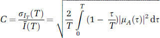
Although the basics of speckle theory have been thoroughly described by Goodman (1965, 1975, 1985, 2006), a short summary of the theory that is important for the validity of biomedical observations is discussed here. The Laser speckle phenomenon is inherently a random interference pattern between multiple independent scattered optic fields produced by coherent light interacting with a surface or medium in which there are relevant imperfections (scatterers). It has long been recognized that the speckle pattern can be modulated by the motion of scattering centres on the surface or in the medium, producing dynamic or time-varying speckle (Dainty, 1975). The first- and second-order statistical properties of the time-varying speckle pattern have led to a number of suggestions for measuring the velocity of the scattering object(s) (reviewed in Briers, 2001). Based on previous studies (Fercher and Briers, 1981; Dunn et al, 2001), the speckle contrast was defined by the ratio of the standard deviation to the mean of a speckle pattern C = σaI/Ī in Goodman's theory (1975). Also from Goodman's results (1985), the relationship between the speckle contrast and the normalized autocovariance function of the temporal fluctuations in the intensity of a single speckle (μ_A(τ) was given by

$$C=\frac{{\sigma }_{I_T}(T)}{\bar{I}(T)}=\sqrt{\frac{2}{T}\underset{0}{\overset{T}{\int }}(1-\frac{\tau }{T})|;{\mu }_A(\tau ){|;}^{2}d\tau }$$

(1)

where the function (1–(τ/T)) is the deterministic autocorrelation function of the CCD exposure window. Generally, researchers have made a tacit assumption that 1–(τ/T)≈1 when the effective exposure time T grows sufficiently large (equation (8), Fercher and Briers, 1981). While T was slow enough for this to be valid two decades ago, much faster CCD cameras are now available that could make this assumption incorrect. This was the first major assumption used in the literature that we tested for validity.

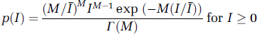
Siegert's relation can be applied for a fully developed speckle if a circular complex Gaussian random process is used as an underlying model (Jakeman, 1973). This relation conveniently links the autocorrelation of the electromagnetic field to the normalized autocovariance of the temporal fluctuations in the intensity of a single speckle, μ_A(0) (Goodman, 1975). The validity of using the assumption of fully developed speckle to derive expressions for μ_A(τ) (and hence equation (1)) has not been tested in biological systems. According to Goodman's theory (1975), the intensity statistics for coherent light illuminating a rough surface is predicted by the gamma probability density function (PDF) p(I):

$$p(I)=\frac{(M/\bar{I}{)}^M{I}^{M-1}\exp (-M(I/\bar{I}))}{\Gamma (M)}forI\ge 0$$

(2)

where M is a shaping constant and Γ(M) is the gamma function. For the special case of M = 1.0, p(I) reduces to a negative exponential, a characteristic signature of fully developed speckle. Therefore, p(I) obtained from our experimental data was examined to assess whether the shaping constant was consistent with fully developed speckle. This would verify whether a circular complex Gaussian random process model is an acceptable assumption in the derivation of equation (1), as is made in the literature. This was our second goal.

Since the speckle image is modulated by the movement of scatterers when a rough surface is illuminated with laser light, μ_A(τ) is of fundamental importance in relating the statistics of the detected intensity to the velocity of moving cells in tissue. Based on a simple physical model for in-plane, straightline and uniform-speed movement, Goodman managed to derive an expression for μ_A(τ) as follows:

$$\begin{array}{rl}& {\mu }_A(\tau )\\ & =(\int \underset{-\infty }{\overset{\infty }{\int }}[\exp ({\sigma }^2{e}^{-(\Delta x^2+\Delta y^2)/r_o^2})-1] \\ & \times [\exp ({\sigma }^2{e}^{-(((\Delta x-v\tau {)}^2+\Delta y^2)/r_o^2)})-1]d\Delta xd\Delta y)/\\ & \int \underset{-\infty }{\overset{\infty }{\int }}[\exp ({\sigma }^2{e}^{-((\Delta x^2+\Delta y^2)/r_o^2)})-1{]}^{2}d\Delta xd\Delta y\end{array}$$

(3)

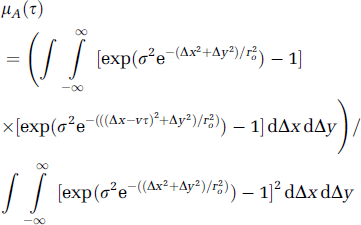
where σ² is the variance of the phase process; r²₀ is the coherent radius; v is the speed of the moving object; and Δx,Δy are spatial locations (Goodman, 2006). To mimic the phase process of photon-tissue interactions, we introduce a classical phase function below. This produces a simple model that allows speed (and hence flow) information to be derived from speckle contrast. It has been demonstrated by Monte Carlo simulation that there is a family of phase functions such as the Henyey-Greenstein functions that are well suited to describe singlescattering events in turbid media like tissue (Henyey and Greenstein, 1941; Wang et al, 1995). The expression for Henyey and Greenstein scattering phase functions was proposed as follows:

$$p(\cos \theta )=\frac{1-g^2}{2(1+g^2-2g\cos \theta {)}^{3/2}}$$

(4)

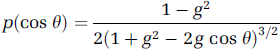
A value of 0.94 for the anisotropy factor g in grey matter has been used (Wang et al, 1995). If the deflection angle θ were assumed to be distributed randomly within the range 0 to π, then we can estimate that the value of σ² is (34 π)² in grey matter by equation (4). Thus, a numerical integration of equation (3) can be performed to get an approximate expression for μ_A(τ), as plotted in Figure 1.

Figure 1

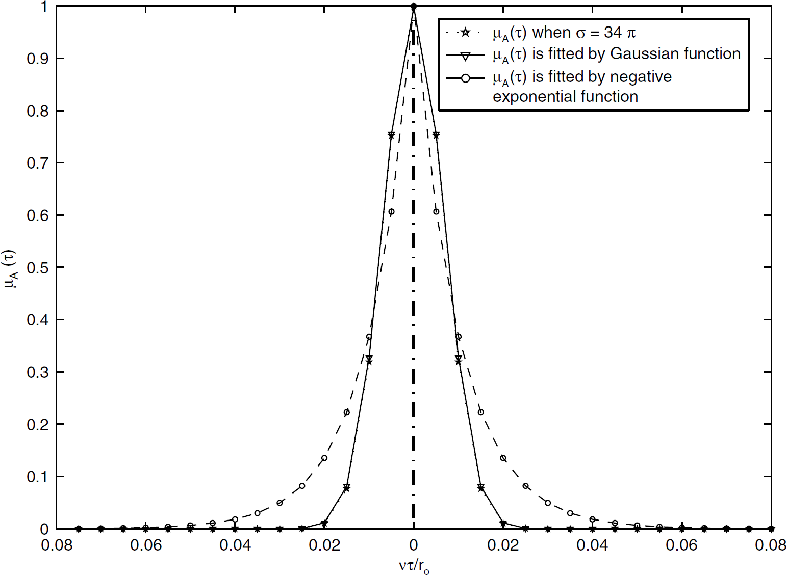
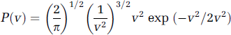
Plot of μ_A(τ) against vt/r_o for Goodman's theoretical model, as well as μ_A(τ) fitted by a negative exponential function (R² = 0.93) and a Gaussian function (R² = 0.99). Here, the value of s was estimated by Henyey and Greenstein scattering phase function (σ = 34π).

Having derived an expression for μ_A(τ) and hence C by substitution into equation (1) (an ergodic random process is assumed for the resultant speckle pattern), we can now compare it with simpler forms that have been previously used in the literature. These simple forms include negative exponential and Gaussian functions that can be substituted for μ_A(τ) in equation (1), giving rise to

$$C=\frac{{\sigma }_s}{⟨I⟩}={\{\frac{{\tau }_c}{T}+\frac{1}{2}{\left(\frac{{\tau }_c}{T}\right)}^2[\exp (-2T/{\tau }_c)-1]\}}^{1/2}$$

(5a)

$$\begin{array}{rl}C=& \frac{{\sigma }_s}{⟨I⟩}\\ =& {\{\frac{{\tau }_c}{T}erf\left(\sqrt{\pi }\frac{T}{{\tau }_c}\right)-\frac{1}{\pi }{\left(\frac{{\tau }_c}{T}\right)}^2[1-e^{-\pi (T/{\tau }_c{)}^2}]\}}^{1/2}\end{array}$$

(5b)

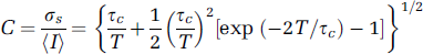
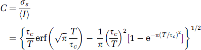
where erf(x) is a standard error function. Plots of equation (5a) and (5b), with and without the assumption that 1 – (τ/T)≈1, can be found in Figure 2. In the Discussion, we compare these simpler forms with the numerically solved expression using equations (3) and (4).

Figure 2

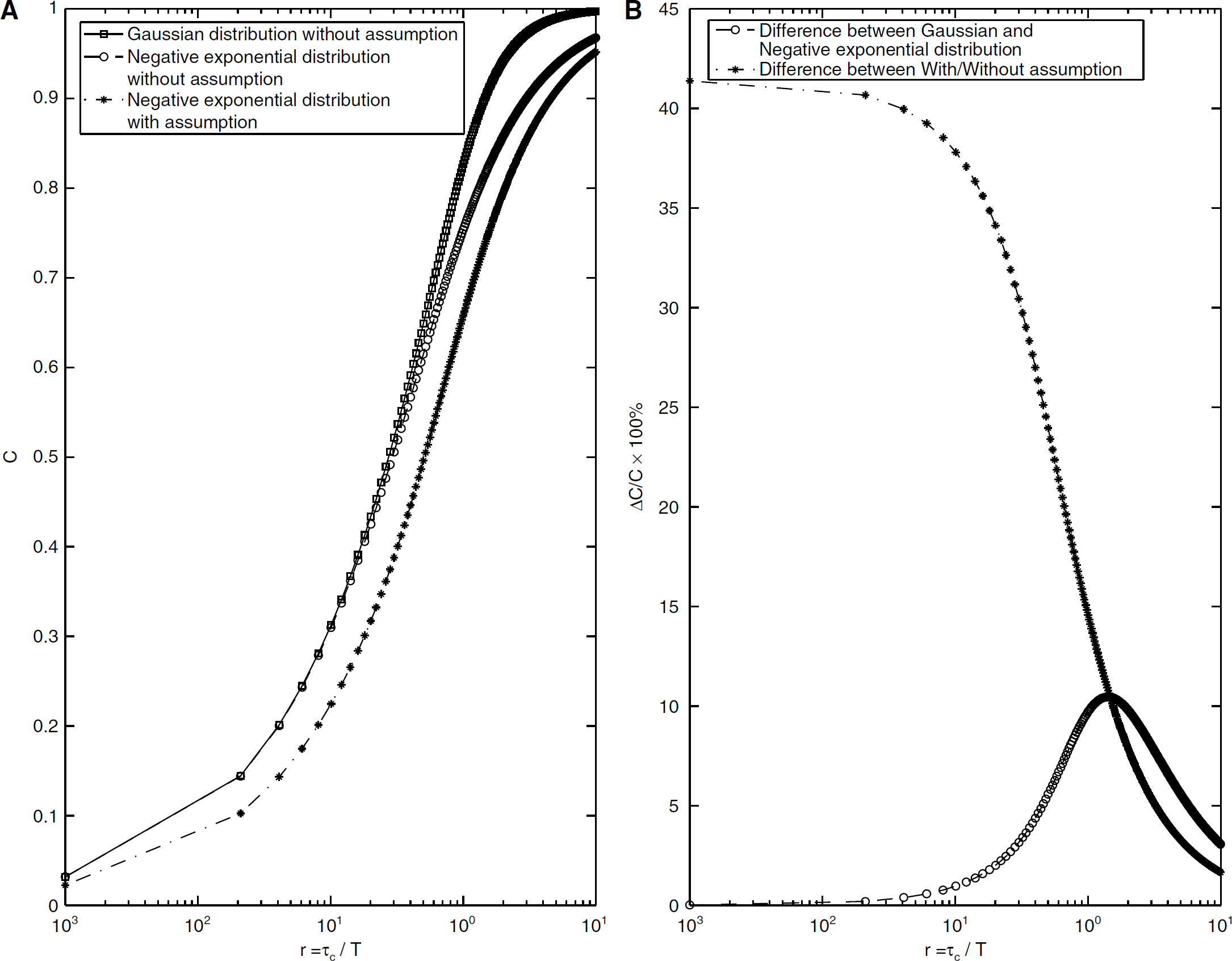
The relationship between the speckle contrast and the ratio r plotted on a semilogarithmic scale. (A) The theoretical curves of the speckle contrast against r were plotted with and without the assumption T»τ_c for the negative exponential function, and without the assumption T»τ_c for a Gaussian function. (B) The % error in speckle contrast with our without the assumption for a negative exponential and for a comparison of the Gaussian versus negative exponential plotted as a function of r.

From Bonner and Nossal's theory of LDF (1981), τc is inversely related to the mean translational speed of the moving blood cells (τ_c≈1/v). Taking advantage of this simple relationship, the mean velocity of the scatterers can be obtained from the numerical solution of τc in the above equations. This mean velocity is an absolute number allowing quantitative flow measurements to be made, in principle. The exact relationship between the correlation time and the velocity will depend on the velocity distribution of the scatterers because it also contributes to determine the shape of the autocorrelation function. In practice, particles (mainly erythrocytes) move in the blood vessels with a variety of velocities, which depends on the vascular size, geometrical distribution, and is spatially regulated by many kinds of chemical and/or neurogenic factors (Sokoloff, 1996). Some kind of velocity distribution function is usually used to statistically describe these velocity attributes, such as the Maxwellian velocity distribution proposed by Bonner and Nossal (1981). In terms of scalar velocity v, the Maxwellian distribution becomes

$$P(v)={\left(\frac{2}{\pi }\right)}^{1/2}{\left(\frac{1}{v^2}\right)}^{3/2}{v}^2\exp (-v^2/2v^2)$$

(6)

where < V² > is the second moment of the distribution. In LSCI, the raw speckle image recorded by the CCD camera is converted into the speckle contrast image using a definition of speckle contrast, in which the flow information has been embodied (Dunn et al, 2001). Therefore, the probability density histogram of the speckle contrast image should reflect the spatial distribution of the velocities within the imaged area. In our study, we also examine this velocity distribution based on our data obtained by manipulating CO₂ to change blood flow in the rat brain.

Materials and Methods

Animal Preparation

Both LDF and LSCI were used to monitor blood flow in the exposed cortex of isoflurane-anesthetized rats. This study was approved by the University of Western Ontario's Institutional Animal Care and Use Committee. Male Sprague-Dawley rats (body weight from 275 to 300 g, n = 6) were housed in a 12 h dark and 12 h light cycle and fed ad lib. Rats were firstly anesthetized with isoflurane (4% induction, 1 to 1.5% maintenance) in an induction chamber with ventilated medical grade room air. A tracheotomy tube was inserted and volume ventilation in air/O₂ performed to normocapnia (PaCO₂ = 32±1 mm Hg). End-expiratory PaCO₂ and respiration rate was monitored during the experiments (Nellcor Puritan Bennett Inc., CA, USA). When performing the carbon dioxide challenge (PaCO₂ range: 22 to 51 mm Hg), the PaCO2 was lowered by hyperventilation and raised by hypoventilation using a dual-mode pressure controlled ventilator (Kent Scientific Corp., CT, USA) (Grubb et al, 1974). At least 15 mins was allowed for the establishment of a steady state at hypocarbic and hypercarbic phases. Under anesthesia, femoral arterial and venous catheters were placed for drug administration, continuous recording of mean arterial blood pressure (MABP), and determination of arterial blood gases, pH and blood glucose levels (SpaceLabs Medical Inc., WA, USA). Arterial oxygen saturation was noninvasively monitored by a pulse oximeter (Benson Medical Industries Inc., Canada). During the experiments, body temperature was maintained between 37.0 and 37.5°C by a rectal probe and servo-controlled heat pad (Gaymar Industries Inc., NY, USA). The cranial window was created using small modifications of our previously described method (Mirsattari et al, 2005). The anesthetized rats were then immobilized in a stereotaxic frame. The animal head was shaved and scalp excised to expose the skull. The skull on one side (~3 × 3 mm2) 1.5 mm anterior to and 1 mm lateral to the bregma was bored with great care to translucency under saline cooling. The thinned skull preparation had the advantage over a full craniotomy since it kept the dura mater intact and allowed a long-term investigation into the changes in the exposed area of cortex within a single animal while preserving the integrity of the brain surface environment. Despite this, bone translucency during prolonged experiments would change. Therefore, several drops of mineral oil were applied to form a thin film on it to prevent drying and improve the image quality. With our system design we performed sequential LSCI-LDF measurements on different trials. A fine needle laser-doppler probe (450 μm diameter, Oxford Optronix, UK) held by a micromanipulator was positioned over the selected small imaging region-of-interest (ROI) in an area devoid of large vessels in the exposed cortex. Microvascular blood perfusion in the rat brain tissue was monitored with an OxyLab Laser Doppler Microvascular Perfusion Monitor (Oxford Optronix) and the data were recorded by PowerLab system (ADInstruments Inc., Toronto, Canada) and stored on a computer for offline analysis. Throughout the entire study, animals always remained intubated and ventilated, and were killed with an overdose of sodium pentobarbital on completion. High-quality anatomical images of each subject were collected as reference when the exposed cortex was evenly illuminated using green light (l = 540±10 nm) via two fiber-optic light guides attached with two collimating lenses (Oriel instruments, Newport, CT, USA).

Laser Speckle Contrast Imaging Instrument

The LSCI instrument described here is similar to that developed by other groups (Dunn et al, 2001), with additional modifications for higher performance. The laser beam from a laser diode (Hitachi, HL7851G, 785 nm, 50 mW, Thorlabs, Newton, NJ, USA) was coupled by two collimating lenses into a 600-mm diameter optical fiber (2 m length). The output beam from the fiber was collimated by the third collimating lens (f = 8 mm), and adjusted to provide uniform illumination on the surface of the exposed brain tissue (~8 mm diameter). Although a long multimode optical fiber could potentially suppress the speckle signal, it has been demonstrated recently that intermodal dispersion was not a critical factor in signal generation by interference under conditions like ours (Petoukhova et al, 2004). During the experiments, the temperature of the laser diode was maintained at 25°C (temperature stability: < 0.002°C) by a precise controller (TED200, Thorlabs). Images were captured by a 16-bit, thermoelectrically cooled CCD camera (PIXIS, Princeton Instruments, NJ, USA) and transferred to a computer by imaging software (WinView/32, Princeton Instruments). A tandem macroscope (Redshirtimaging LLC, CT, USA), which could provide variable numerical aperture (NA, 0.06~0.4) for low magnification (x 0.75~5) and long working distance (1.0~4.0cm) and large field-of-view (FOV), was coupled with the CCD camera to focus the images and adjust the speckle size. One vital factor in LSCI is the determination of speckle size, which could affect the final spatial resolution of LSCI. In imaging speckle geometry, the speckle size in the imaging plane should match the size of detector elements (13 × 13 μm² here) to avoid the spatial averaging that would suppress the speckle pattern and destroy the speckle contrast. Like previous studies, the size of the speckle observed in the image plane was approximately calculated by d = 2.44ΛMf. Here Λ is the illumination wavelength, M is the magnification of the macroscope system, and f is the f-number of the camera lens. In this study, f is approximately 9.4 at a wavelength of 785 nm. The CCD camera with the macroscope lenses was mounted on our custom-designed platform and positioned vertically to obtain the whole view of the animal head. Extreme care was taken to isolate the camera and the laser path from stray light noise contributions to the speckle image.

Data Acquisition and Analysis

Since LSCI exploits the spatial statistics properties of laser speckle to obtain the two-dimensional velocity distribution by analyzing the spatial blurring of the raw speckle images, any other blurring effects because of spatial and/or temporal averaging could reduce the speckle and cause errors in estimating the relative changes of blood flow in the experiments. Moreover, the sensitivity to in-plane motion of LSCI is also determined by the speckle size (Briers, 1996). As we mentioned above, the temporal averaging also imposes the same effect on the speckle, such that a long exposure time compared with the correlation time of the moving scatterer could average out the speckle. A small ROI (~ 250 × 400 pixels) subset of the full FOV (1024 × 1024 pixels) was selected to record the raw speckle images. At each PaCO₂ steady state, 200 speckle images were acquired at 2 Hz. Six to seven trials were repeated on an animal in alternating order of hypercapnia and hypocapnia. When changing PaCO₂ to a new steady state, the laser beam was blocked by a shutter to avoid unnecessary irradiation to the exposed brain tissue. The first raw speckle image at each level of PaCO₂ was used as a baseline to normalize the image set and discarded from later analysis. Each of the remaining 199 images of the normalized image set were used to produce the distribution function of measured speckles and the averaged distribution, which were then compared with the p(I) distribution from equation (2). To convert the variations of speckle contrast to the intensity variations, a small area on the raw speckle image was chosen in which a sufficient number of speckles were expected. For our settings (25 ms exposure time plus 475 ms delay time), it is reasonable to believe that speckles in sequential images are not correlated (as there is significant movement of the scatters in that time) and hence a 3 × 3 template was used so that spatial resolution was not compromised (Volker et al, 2005). The numerical integrations and other data processing in this study were performed using MATLAB (The MathWorks, Natick, MA, USA). No digital filters were applied to remove image noise and the final effective spatial resolution was 18 μm/pixel. Only the speckle contrast images within one CO₂ steady state were averaged, which has been proven effective in minimizing drift effects of systemic physiological factors (heart-beat, respiration, blood pressure and spontaneous oscillations of pulsatile blood) (Detre et al, 1998). The histogram of the speckle contrast image made by averaging one image data set was fit with a Maxwellian distribution. Numerically solving τc from equation (6), the relative velocity maps of CBF were calculated in arbitrary units simply by inverting tc. To compare the velocity changes sequentially measured by both LSCI and LDF measurement in the same area, the CO₂ reactivity index was defined by the following expression in units of %/mm Hg:

$$\begin{array}{rl}& {CO}_{2}reactivityindex\\ & =\frac{(CB{F}_{{changingCO}_2}-CB{F}_{base{CO}_2})/CB{F}_{{baseCO}_2}}{PaC{O}_{2{changingCO}_2}-PaC{O}_{2{baseCO}_2}}\times 100\end{array}$$

(7)

where CBF_changingCO2 is the flow or velocity obtained by LDF or LSCI during PaCO₂ was changed to a new level; CBF_baseCO2 is the flow or velocity during the baseline level.

Theoretical and Experimental Results

We first consider the numerical integration of equation (3), giving μ _A (τ) as presented in Figure 1. If the variance of the phase process that gives rise to the speckle pattern increases, μ _A (τ) will be narrower. This is usually the case in biological tissues, where the coherent light source can penetrate the tissue and interact with the vasculature below the surface, giving rise to speckle contrast values that are generally quite small (C < 0.2). Moreover, when the velocity v increases while other parameters remain fixed (vτ being distance moved in equation (3)), the value of μ _A (τ) will decrease such that the speckle contrast C reduces too. This is why fast flowing vessels appear darkest in LSCI and why even tissue areas perfused with capillaries gets darker with increases in blood flow such as in our hypercapnia experiment (Figure 4). Owing to the complicated nature of more realistic forms of μ_A(τ) such as we have chosen in equation (3), the negative exponential function is commonly used to fit its shape and indeed it provides a good approximation to μ _A (τ) within the range (R² = 0.93, shown in Figure 1). However, a Gaussian function is found to almost perfectly match with the calculated μ_A(τ) (R² = 0.99). Particularly at the centre of the autocorrelation function, it is a much better fit to μ _A (τ) compared with the negative exponential function. The implications of using both Gaussian and negative exponential functions to replace μ _A (τ) in equation (1) were explored in this study.

Figure 3

(A) Histogram depicting the probability density function of the measured speckle pattern under 32 μm Hg PaCO₂. The error bars associated with this histogram were calculated from one image data set (the first speckle image was discarded). (B) An illustration of the theoretical Gamma distributions (M =1.0 and 1.2) and normalized PDF from the left histogram. They both presented a strong correlation with the PDF measured from our experiments, respectively (R² = 0.96 and 0.98).

Figure 4

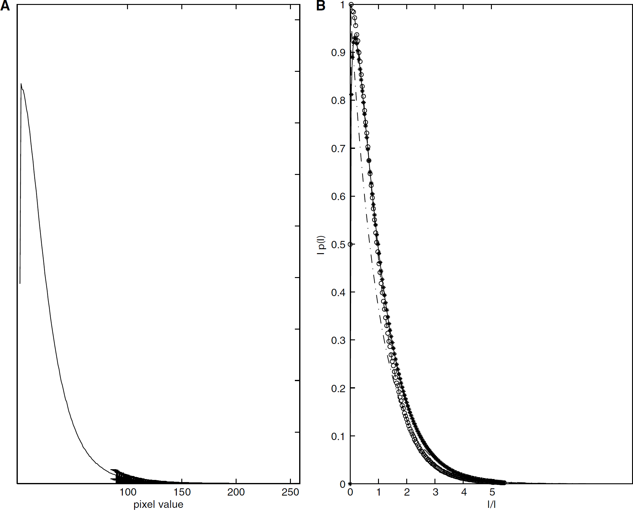
Speckle contrast images (top row) and their corresponding histograms (bottom row) under three different levels of PaCO₂ (27, 32 and 50 μm Hg). The Maxwellian PDF was scaled to fit the histograms of speckle contrast images at different levels of PaCO₂, in which the values of < v² > were 164, 154 and 84 respectively. The R² values of each fit were 0.97, 0.97 and 0.95.

As we have discussed in the Introduction, previous studies typically assume that 1–(τ/T)≈1, that is, that (μ/T) is small. Therefore, the integral window 1–(τ/T) in equation (1) is replaced by a square function that is unity. Figure 2A shows the solution to equation (5a) and (5b) as a function of the inverse of the velocity of the scatterers. For the case of a negative exponential function (equation (5a)), we have plotted the speckle contrast C both assuming 1–(τ/T)≈1 and using the full form 1–(τ/ T). For a measured speckle value C, it is clear that different velocities can be inferred from the different curves. Under the conditions that the full integral window is used (1–(τ/T)), there is no difference in the velocity inferred from using the Gaussian form of μA(τ) and the negative exponential form of μ _A (τ) for imaging parameters used in most studies. However, if the assumption 1–(τ/T)≈1 is used, then the negative exponential form of μ _A (τ) leads to a significantly different inferred velocity. Figure 2B shows the percent errors that can arise in the speckle contrast, as a function of (τ_c/T). For the biologically relevant situations currently used for LSCI, the figure shows that a significant error in C (up to ~41.8%) could be caused when making the assumption 1–(τ/T)≈1 on the integral window. Similarly, a 10.5% difference could be introduced by applying different functions to model μ_A(τ) even though the same subject was imaged.

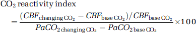
The intensity histogram of the pixel frequency against the intensity values of the raw speckle images in one data set at 32 μm Hg PaCO₂ was plotted in Figure 3A. The error bars were calculated from the 199 images of one trial (the first image was discarded). The normalized PDF from the measured speckles was computed from this averaged histogram and was displayed as a semilogarithmic plot in Figure 3B along with Īp(I) as a function of I/Ī for M =1.0 and 1.2.

Figure 4 showed one set of speckle contrast images (220 × 326 pixels) and their corresponding histograms, in which (A), (B), and (C) are the images made at different levels of PaCO₂: 27, 32, and 50 μm Hg, respectively. Noticeable darkening in the tissue areas occurs as the flow increases between normocapnia and hypercapnia. Additionally, a clear increase in the diameters of pial blood vessels in hypercapnia occurs (Figure 4C). The histograms of speckle contrast images corresponding to the three levels of PaCO₂ in the same animal were calculated and fitted with Maxwellian PDFs. On comparison with these three distributions, a small shoulder that can be clearly observed at 27 μm Hg disappeared as the carbon dioxide pressure increased to 50 μm Hg. The pixels that formed this small plateau originated from the microvascular bed (no large visible vessels). Additionally, the histogram at high CO₂ level (50 μm Hg) was better fit to a Maxwellian PDF with a smaller value of < V² >, which meant the distribution of the CBF during higher PaCO₂ was more homogeneous than normocapnia. This finding was consistent with previous conclusions (Vogel et al, 1996; Hudetz et al, 1997; Ayata et al, 2004).

Based on the speckle contrast images, the velocity maps were calculated from equation (5) in arbitrary units, using the negative exponential form. The ratio of the velocity map at PaCO₂ of 50 μm to that at PaCO₂ of 32 μm was calculated (Figure 5A). The ratio of the velocity map at PaCO₂ of 32 μm to that at PaCO₂ of 27 μm was also calculated (Figure 5B). This latter map showed very little change in blood flow. Correcting for an additional factor of 2 that was missing in the form of equation (1) used by others in the literature (Fercher and Briers, 1981), our absolute value maps of the velocity are almost twice that of those previously reported in the literature. However, the relative changes of blood flow maps between the two PaCO₂ levels showed no significant difference to literature values, since a 25-ms exposure time gives a value of the integral window autocorrelation function that approaches 1 in this case (see equation (1)).

Figure 5

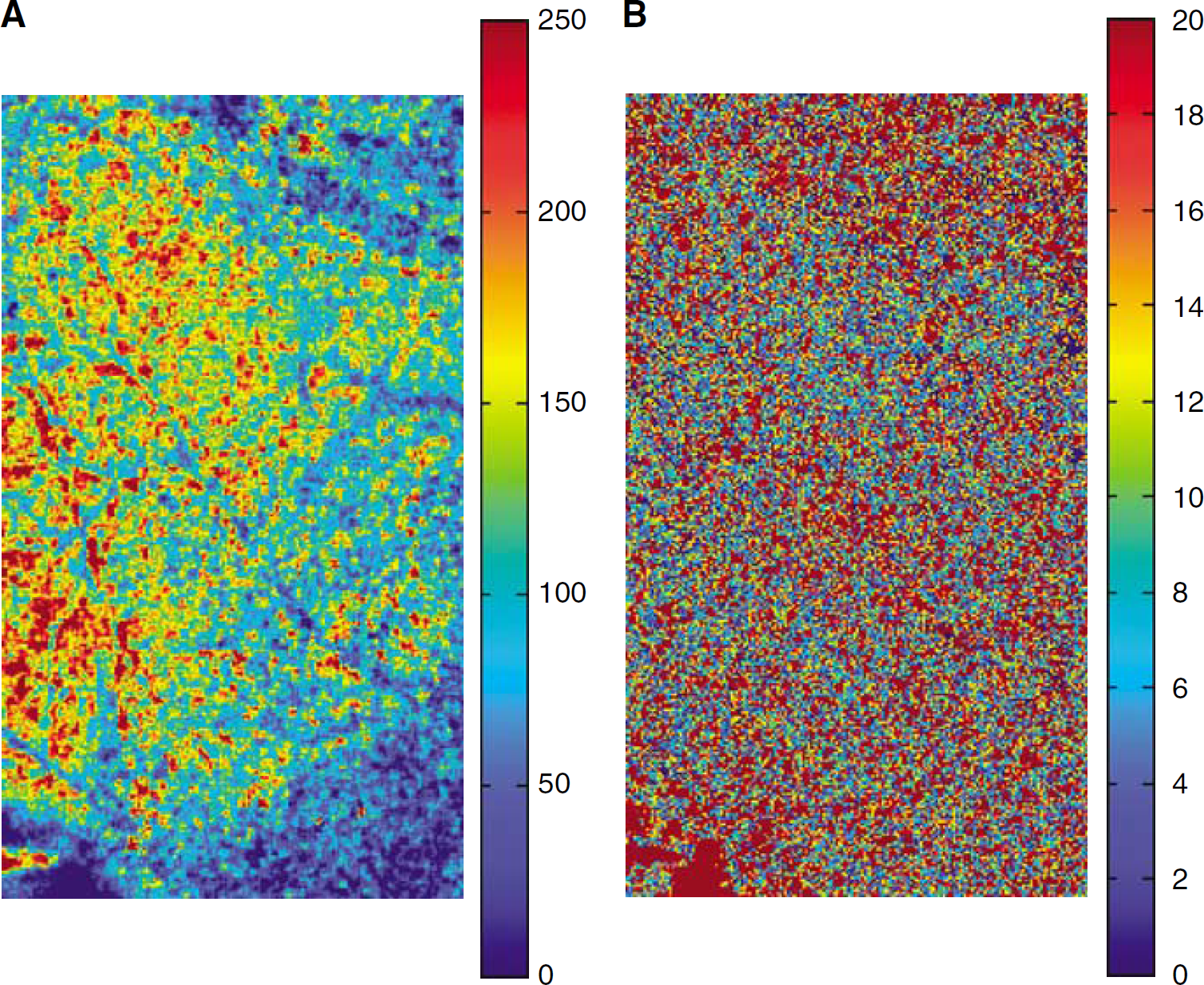
Relative velocity maps calculated from the above speckle contrast images were shown as percentage change against baseline (32 μm Hg) and displayed as pseudocolor images. (A) Relative velocity increase between 50 and 32 μm Hg. (B) Relative velocity decrease between 27 and 32 μm Hg.

The relationship of the CO₂ reactivity index obtained by LSCI and LDF from all the trials was demonstrated as the plot in Figure 6. The results from LDF measurements showed a high correlation (R² = 0.92) with LSCI measurements in the same area under the conditions that the PaCO₂ was lowered or raised. Under our experimental conditions, the use of either equation (5a) or equation (5b) did not make any difference (< 0.1%) to the calculation of the relative velocity, Thus, the results from equation (5a) (negative exponential function) were used to compare with that of LDF and are comparable to previous studies (Dunn et al, 2001; Ayata et al, 2004; Kharlamov et al, 2004).

Figure 6

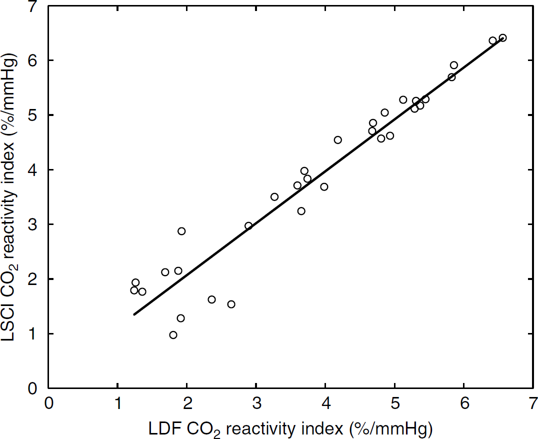
The relative changes in blood flow during the stimulation induced by carbon dioxide change measured by LSCI demonstrated strong correlation with the results on LDF on the same area (R² = 0.92).

Discussion

Our theoretical analysis and preliminary results from animal experiments show that the ‘mistakes’ pointed by Bandyopadhyay and his co-workers in the LSCI theory of Fercher and Briers did not produce any significant errors under our experimental conditions using relative flow changes, although these errors are in fact real. However, the original LSCI theory of Goodman contains the correct formulations of the problem that were lost over the years.

It is important to distinguish between the optical spatial resolution of LSCI and the functional spatial resolution for LSCI. It is well known that regional CBF exhibits a significant degree of spatial heterogeneity not only at the microscopic but even at the gross anatomical level (Sokoloff, 1996). Results recently reported by Yuan et al (2005, see Figure 4 in there) show a higher sensitivity to microvascular blood flow changes at a 20 ms exposure time compared with 5 ms. They attribute this to the sensitivity of the CCD camera, but our analysis shows that shorter exposure times are intrinsically not as sensitive to the microvascular blood velocities because of the underlying physics. Our analysis shows that the choice of exposure time determines the sensitivity to microvascular velocities, and hence the functional spatial resolution. Longer T values give enhanced sensitivity to the microvasculature, which in turn allows mapping of a signal that is more co-localized with neuronal changes in applications such as mapping of cortical function. The velocity of the eythrocyes in the microvasculature corresponds to a τc value that is higher than in the pial vessels. To optimize C from the microvasculature, T must therefore be chosen longer than it might be for larger vessels. Thus, this tradeoff should be made as appropriate for the experiment being considered. In our experiments, pial vessels were robustly detected. We found that no blood vessel became visible during hypercapnia (>96% trials in this study) that was not visible under normocapnia with the 18 μm spatial resolution used. The contrast between the tissue with its unresolved capillaries and the pial vessels was highest in the 27 μm Hg PaCO₂ condition. The tissue significantly darkened at 50 μm Hg PaCO₂, but the same pial vessels were still visible. The tissue darkening we saw is more striking than in previous studies, as the 25 ms exposure time increases the sensitivity to the flow in the microcirculation. Thus, exposure times of this order would be needed to study the microcirculation signal that is presumably most tightly coupled to the neural activity.

There is no doubt that LSCI is a promising, quantitative, minimally invasive method to achieve in vivo high-resolution (submillimeter) visualization of blood flow in exposed biological tissue. However, there is still considerable room for optimizing this imaging technique. Several issues need to be addressed in the future work.

Firstly, the nonlinear relationship between τ_c, T and C based on the simplified model is heuristic here, making it empirically hard to characterize. It depends in a very complicated manner on the experimental object and physiological conditions including the thickness of the thinned skull, all of which would particularly affect the practical range of τc that can be observed because of sensitivity, scatter etc. (Ayata et al, 2004). In future studies, it would be of great interest to define the specific profile of μ _A (τ) with respect to the cell speed distribution from in vivo experiments so that a more accurate association between the velocity and speckle contrast could be formulated. In principle, it is possible to recover the cell speed distribution from the measured contrast of the speckle pattern if the specific profile of μ _A (τ) is known (Stern, 1975). Thus, the velocity of blood flow measured by this technique might be made more quantitative.

Secondly, close inspection of the histograms as shown in Figure 3B reflects some departure of the measured PDF from the ideal negative exponential curve (M =1) for fully developed speckle. We find that a shape factor of M= 1.2 fits the measured PDF very well (R² = 0.98). It is possible that fully developed speckle is not a perfect model of coherent light interacting with a brain. Also, various measurement noise sources could contribute to this nonunity value, such as the dark current of camera detector, amplifier noise, background radiation and depolarization effects. Similar findings have been reported by other researchers (Briers et al, 1999; Webster et al, 2003). In our setup, the hardware noise from the CCD has been carefully controlled. The system read noise was typically 9e⁻ r.m.s. and the dark current was less than 0.003e⁻/p/s when the camera was operated at −70°C. Thus, no dark current correction was applied in our study. The wide dynamic range of CCD camera, averaging strategy and the experiment paradigm applied here helped us to effectively accommodate the contamination from various noise sources. It remains to be seen whether the difference between M= 1 and 1.2 is because of the instrumentation or the photon processes in the biological system.

Thirdly, although our results demonstrate for the first time an experimental verification of the Maxwellian distribution used by Bonner and Nossal in their theoretical formulations, this problem deserves more attention. The model we used in this study has been extensively studied since Kety and Schmidt in 1948 where an increased homogeneity of the velocity distribution during hypercapnia was expected (Hudetz et al, 1997). This behavior of CBF responses was indeed embodied exactly as the results from our fitting with Maxwellian distribution (Figure 4). The Maxwellian is broadly considered the best form to describe a stable velocity distribution at an equilibrium state such as the physiological conditions of our animal model. And all the images obtained and shown throughout this study actually characterize the behavior of CBF during the steady state. If the system has a strong anisotropic flow, a Maxwellian distribution may be not appropriate anymore. We have presented a way to experimentally measure the distribution if necessary.

One caution in any animal experimental procedure should be noted here. Stable anesthesia over long durations (many hours) generally requires mechanical ventilation and invasive blood gas sampling, which is relatively difficult to perform with the use of α-chloralose as an anesthetic (Duong et al, 2001). Our group recently demonstrated that the rats under isoflurane anesthesia are stable over prolonged and repeated fMRI measurements (Mirsattari et al, 2005; Mirsattari et al, 2006). However, isoflurane does cause a significant reduction in the systemic vascular resistance compared to α-chloralose, with a marked increase in basal CBF (Matta et al, 1999; Ayata et al, 2004). Thus, other physiological vital signs have to be continuously monitored throughout this type of experiment. Furthermore, isoflurane depresses cerebrovascular reactivity to CO₂ relative to awake conditions (Sicard et al, 2003), which might explain why the CBF change between 27 and 32 μm Hg was less pronounced (Figure 5B).

Laser speckle contrast imaging has become an increasingly popular technique to visualize blood flow response to external functional stimulation since Dunn and co-workers' first application on the rat's brain (2001). It can be anticipated as a complementary method to intrinsic optical imaging techniques that depend on the change in concentrations of intrinsic chromophores due to oxygen metabolism during functional activation (Grinvald et al, 1986).