Noninvasive Fluid Property Measurements Using Acoustic Methods

Abstract

The properties of a fluid are normally determined using invasive methods. These methods may lead to possibly contaminating or consuming the sample. When only very small amounts of a valuable sample exist, noninvasive measurement methods are preferred. The properties of fluids can then be used to deduce additional properties based on known relationships. In one case, the surface tension of a fluid may be used to determine the concentration of a fluid. We describe a measurement technique involving excitation of the surface of the fluid and the measurement of its response. An acoustic wave is used to both excite and monitor the surface of the liquid. This technique is used to determine the concentration of DMSO and water in solution, and the result determines the amount of fluid needed to deliver an accurate amount of solute in solution. (JALA 2006;11:188–94)

Introduction

The principle of using acoustic waves as a noninvasive measurement method has been around since the early 1900s. Sonar techniques were studied beginning in 1910 and had been used extensively in World War II. ¹ Ultrasound is used today to reconstruct the surfaces of organs inside the human body. ² By sending sound waves into a body, the reflections of those waves may be used to reconstruct the change in density inside the body.

Acoustic dispensing technology is based on the use of focused concentrated acoustic energy on the surface of a liquid to eject a droplet of liquid from the well. When the impedance of two materials is very different it causes a high percentage of acoustic energy to be reflected. The reflection of this energy has the effect of applying pressure to the interface between these two materials. When one of these materials is liquid and the other material is the atmosphere, the pressure on the surface of the liquid will cause that surface to rise. By using this applied pressure in a concentrated area, controlled volumes of liquid may be ejected from the surface of the liquid. This technology was described by Xerox in 1989, ³ and this technology was described in conjunction with the application of ink printing at the Ultrasonics Symposium in 1992. ⁴

EDC Biosystems has incorporated this technology into the ATS-100 liquid-handling tool. This tool uses acoustic energy to dispense liquid droplets from one well plate to an inverted well plate placed over the top. By applying enough pressure to a specific area on the surface of a liquid, the surface is pushed upward until the restraint of the surface tension is broken and a droplet is ejected. By changing the force, duration, and area of the effected surface, the volume of the droplet ejected may be adjusted. However, because the surface tension restrains the surface and the viscosity of the liquid affects the velocity of the fluid, these parameters are important in accurately determining the volume of a drop ejected.

Methods and Materials

All of the measurements for this paper were made using the EDC Biosystems HTS-01 liquid transfer tool with modifications to the software to enable specific data collection techniques. The microplates used were Aurora Discovery ChemLib 1536-well microplates. These plates are made out of cyclo-olephin co-polymer. The depth of each well is 4.85 mm, and its diameter varies from 1.36 mm at the bottom to 1.70 mm at the top.

The setup for the four experiments described in this paper centered on the EDC Biosystems acoustic transfer technology. This technology consists of a device that generates acoustic waves that pass through to an acoustic lens which focuses the beam (Fig. 1). This acoustic beam passes through a fluid that acoustically couples the beam to a microtiter well plate that contains the fluid of interest.

Figure 1.

Acoustic transducer geometry.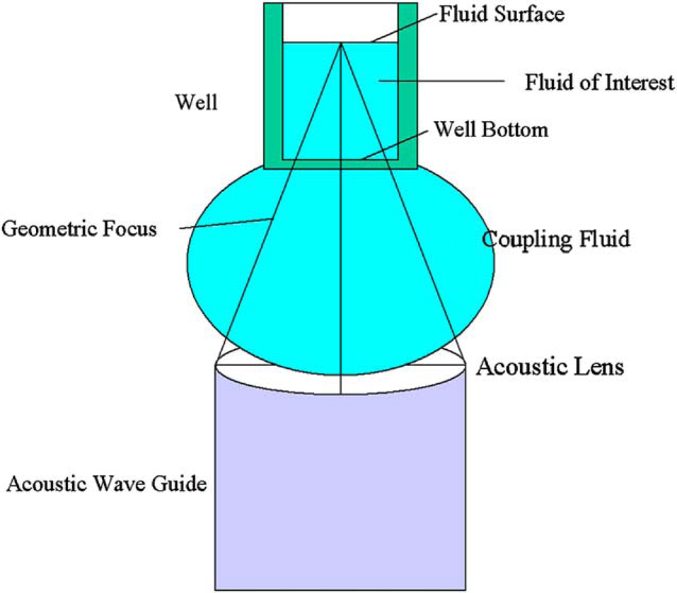

Because the beam needs to be focused on the surface of the liquid of interest, the depth of the fluid in the well needs to be known. This is accomplished by using a sonar technique, that is, to send a short low-energy “ping” toward the surface of the liquid of interest, and measure the time that it takes for the “ping” to reflect off the surface of the liquid and be received at the point in which the “ping” was generated. By using the speed of sound for a “typical liquid”, the distance may be measured and the acoustic transducer is moved into focus.

This technology has been modified in various ways to make the additional measurements required for this experiment.

1. (1)

   For the speed of sound measurements in experiment 2, the depth of the liquid in the well has been forced to be exactly the depth of the well by placing a microscope slide over a filled well.

2. (2)

   For the surface stimulation measurements, multiple “pings” are generated one after the other to make multiple measurements as the surface of the liquid is moving.

Concepts and Equations

A comprehensive source of information on the application of acoustic energy in the context of these studies may be found in “Acoustic Waves”. ⁵ This text goes into the details of generating, guiding, focusing, and reflecting acoustic waves. For the purpose of this paper, the concept of waves traveling through a medium and their reflection are key issues.

It should be understood that acoustic waves travel through a medium at a particular speed, known as the speed of sound for that medium. Similarly, there is a characteristic impedance of a medium given by the acoustic velocity multiplied by the density of the medium

$$Z_0\hspace{0.17em}=\hspace{0.17em}V\rho$$

(1)

And, when there are two media with an acoustic wave passing from one to the other, the transmission and reflection power amplitudes are given by

$$\begin{array}{c}{R}_{\text{P}}={\left|\Gamma \right|}^2\\ T_{\text{P}}=1-{\left|\Gamma \right|}^2\end{array}$$

(2)

where

$$\Gamma \hspace{0.17em}=\hspace{0.17em}\frac{Z_{02}-Z_{01}}{Z_{02}+Z_{01}}$$

(3)

This illustrates that when acoustic impedances differ greatly, there are large amounts of acoustic power reflected, and when the acoustic impedances are similar, more energy is transmitted.

With this knowledge, one is able to design a device that focuses acoustic energy through a coupling fluid and into a source well plate containing a fluid of interest. With enough focused acoustic energy, droplets may be ejected from the surface of the fluid of interest. However, with less acoustic energy the surface of the fluid of interest may be stimulated as if it were a drum head and the surface will oscillate. The equations that describe this drum model of the surface may be found in Appendix A.

Once the surface of the fluid has been stimulated, its movement can be measured. This is accomplished by measuring the position of the surface at regular intervals. The surface is measured by using a standard sonar technique. A short burst of sound is transmitted, and the reflections from that short burst are timed. Based on the speed of sound through the different materials, the distance can be calculated. If a short burst and pause are generated and the reflections are detected, the distance can be measured repeatedly as the surface is moving. The result is a sample of the position of the surface after each measurement.

Once the oscillation of the surface has been detected, one may separate the three different modes of oscillation by frequency using a Fast Fourier Transform (FFT). The Inverse Fast Fourier Transform (IFFT) can be performed on the separated frequencies yielding three decaying waveforms.

The surface of the fluid may be described as a circular membrane. The oscillation modes of a circular membrane have been studied extensively. These modes of oscillation can be summarized as symmetric and asymmetric modes. If the circular membrane is excited in the center, then the symmetric modes are excited and the asymmetric modes remain quiet.

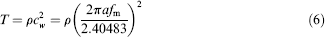
When the circular membrane is stimulated, several symmetric modes of vibration begin to oscillate. The lowest frequency mode is known as the (0,1) mode. The frequency of this oscillation is dependent on the diameter of the well and the surface tension of the fluid in the well. The higher the surface tension and the smaller the well diameter, the higher the frequency of oscillation. The (0,2) and (0,3) modes also contribute to the symmetric oscillation of a circular membrane. The (0,2) mode oscillates at 2.295 times the frequency of the (0,1) mode. The (0,3) mode oscillates at 3.598 times the frequency of the (0,1) mode.

Similarly, when these three modes are stimulated the amplitudes will decay in a short time. How fast these oscillations decay is partially dependent on the viscosity of the fluids on both sides of the membrane: the air and the fluid in the well.

Measurements

Experiment 1—Liquid Level

The amount of liquid in a well may be measured by a sonar technique. A small burst of acoustic waves is directed toward the target, the surface of the liquid, from below. The sound waves travel through a coupling fluid, through a well plate bottom and through the liquid. The speed of sound, c, in a liquid is given by the following relationship between the time t that a pulse takes to travel a distance d through a given liquid

$$c=\frac{d}{t}$$

(4)

Or, by solving for distance d for a known fluid with a given speed of sound c_k, the depth of the liquid in a well may be determined by measuring the time between the pulse received from the reflection of the pulse off the bottom of the well/liquid surface and the pulse received from the reflection of the pulse off the liquid/air surface. Because the second pulse travels twice the distance of interest, the depth of the liquid, the time is twice what is expected

$$d=\frac{c_k{t}_m}{2}$$

(5)

The sound waves are then reflected off the surface of the fluid and back toward the source. Using the speed of sound of the liquid in the well one may use the difference between the time when the pulse is generated and the time when the pulse reflection is received to calculate the depth of the liquid in the well.

Liquid Level Results

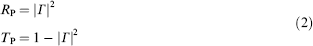
The sensitivity of our liquid level measurements can be demonstrated by draining a well. A well can be drained by ejecting a drop of a known volume from the same well over and over again. Before each drop ejection, the level of the liquid in the well is measured. The drops are indexed as they are dispensed. By graphing the liquid level measured for each drop on the y-axis and the drop index on the x-axis we may show the repeatability of the measurement (Fig. 2).

Figure 2.

Draining experiment.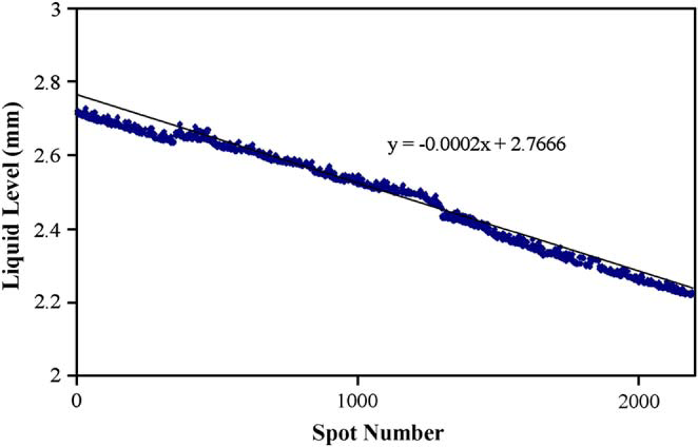

Experiment 2—Speed of Sound

From Eq. (4) the distance measured is equal to the speed of sound multiplied by the time the pulse takes to traverse the distance. Therefore, the speed of sound for the material can be measured if the volume of the fluid and the shape of the container are known. By using several wells filled to a known level and measured several times, a very reasonable measurement of the speed of sound can be determined.

The speed of sound for a fluid in a microplate is determined by measuring the time it takes for an acoustic pulse to travel a known distance through a fluid in a well. This is demonstrated by using several concentrations of DMSO and water. The wells are filled to the top, and a microscope slide was placed over the top to prevent evaporation and provide a reliable flat surface at a known distance. Then the time for the pulse to reflect off the surface is measured. By measuring the pulse travel time multiple times a good determination of the speed of sound for a fluid is possible.

The speed of sound of a DMSO/water solution was measured at several concentrations from 100% DMSO (v/v) to 65% DMSO and 35% water by volume. The fluid is placed in a well to slightly overflowing. A glass cover slide is then placed over the well displacing the fluid and preventing any air from being trapped. In this situation, the depth of the well is known precisely based of the construction of the microplate. The travel time of the pulse and the speed of sound for each concentration are measured (Fig. 3).

Figure 3.

Speed of sound measurement.

Experiment 3—Surface Tension

The surface tension may be determined by stimulating the surface of the fluid, continuously measuring the position of the surface, and detecting the oscillation (Fig. 4). The frequency of the oscillation is related to the tension of the membrane, on the surface of the fluid, which has been described above. This relationship is shown in Eq. (18) in Appendix A. By measuring the frequency of the first mode of oscillation and solving Eq. (17) in Appendix A for surface tension we have

$$T=\rho c_w^2=\rho {\left(\frac{2\pi a{f}_m}{2.40483}\right)}^2$$

(6)

Figure 4.

Raw surface oscillation measured at the center of the surface.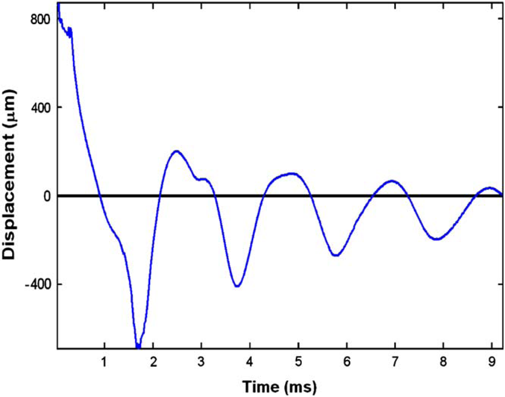

where f_m is the frequency measured.

In general, three modes of oscillation are excited when the surface is stimulated in the center of the well surface. An FFT is performed on the data (Fig. 5), and the values of the three frequencies are extracted.

Figure 5.

Frequency spectrum of surface oscillations.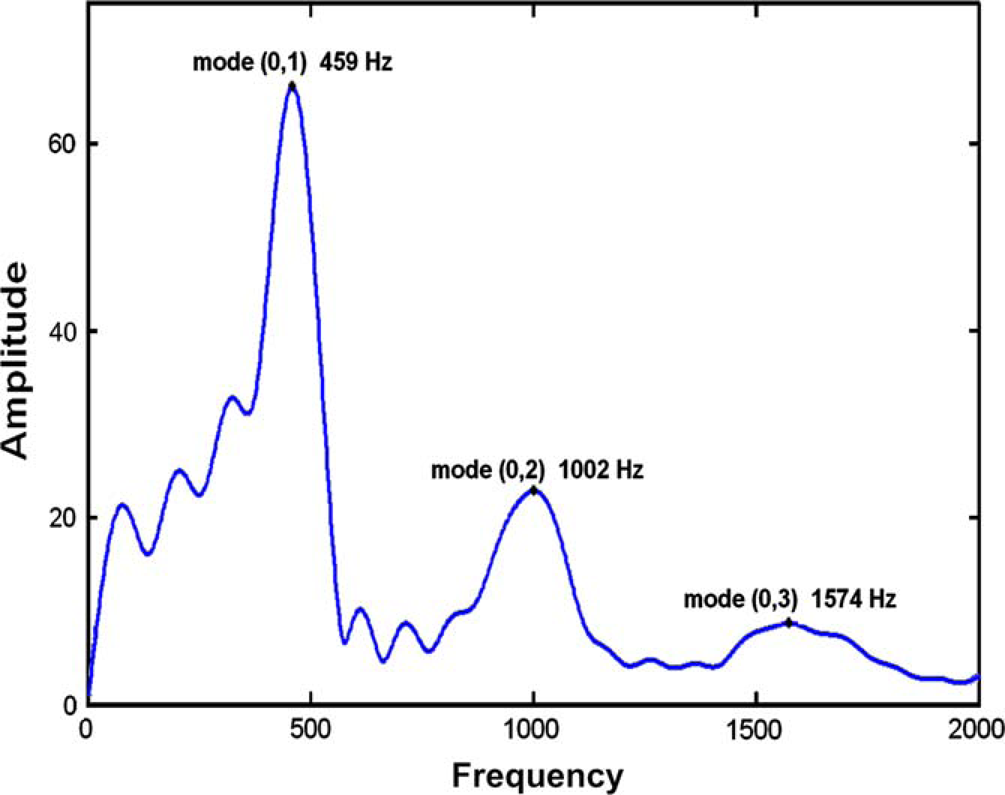

A microplate is filled with different DMSO concentrations at different liquid levels. Data are taken at each well location, and the oscillation frequency of the (0,1) mode is determined for each well. The relationship between the depth of fluid in the well, the concentration of DMSO in water, and the frequency of oscillation is shown (Fig. 6).

Figure 6.

Frequency of mode (0,1) versus liquid level.

Experiment 4—Viscosity

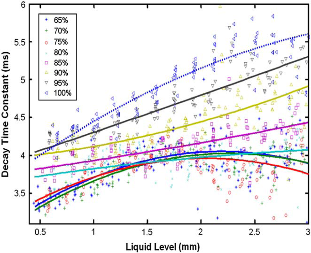
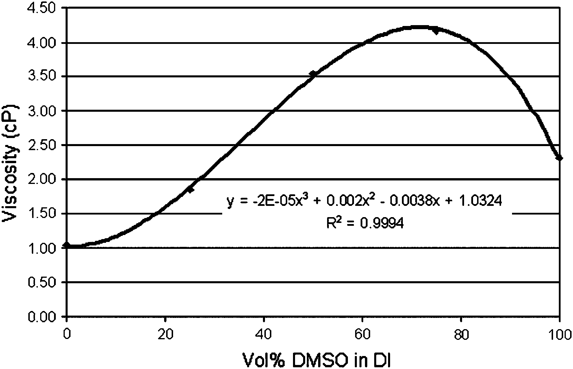
Viscosity may be determined by measuring the dampening of the oscillation. By selecting the data in the FFT plot around the (0,1) frequency peak, the time domain data can be reconstructed using an IFFT. The result is reconstructed (0,1) waveform extracted from the data using the IFFT (Fig. 7). The absolute values of the peaks are fitted to an exponential function. The decay coefficient τ is then plotted for different fluids as a function of liquid level (Fig. 8). This coefficient is related to the viscosity based on Eq. (11) in Appendix A. This shows that the damping of the vibration of the surface is proportional to the viscosity of the fluid. This result may be compared to the measured viscosity of DMSO as a function of concentration (Fig. 9).

Figure 7.

Surface oscillation decay.

Figure 8.

Decay time of mode (0,1) versus liquid level.

Figure 9.

Viscosity versus vol% DMSO in DI water.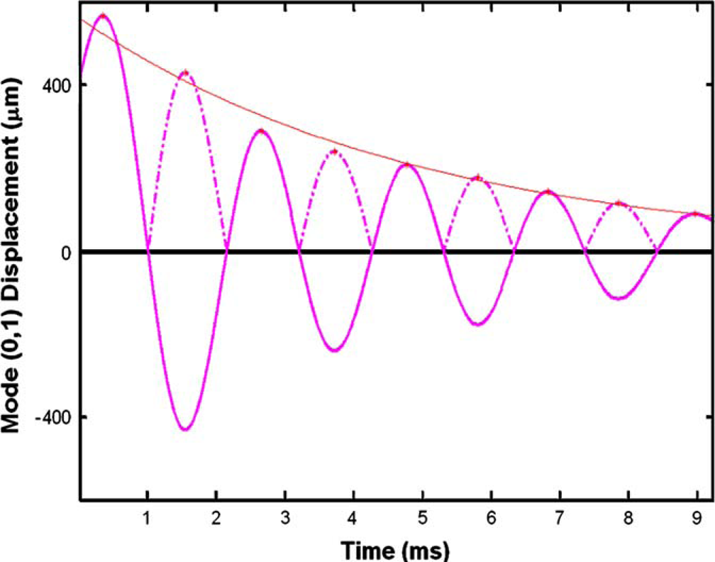

Results and Discussion

The EDC Biosystems ATS-100 liquid handling tool noninvasively measures the fluid properties. One aspect of DMSO is the tendency to absorb and evaporate water depending on the humidity of the environment. Therefore, if atmospheric water is absorbed by the DMSO containing a compound solute, the amount of compound solute transferred is reduced by this absorption. Similarly, if water evaporates out of the DMSO compound solution, then an increased amount of compound solute would be transferred. In response to this problem, EDC BioSystems has integrated the measurement of DMSO concentration into its tool based on the measurement of surface tension and viscosity of a compound solution. By using this technology, EDC BioSystems is able to compensate for the change in concentration and eject the proper amount of compound solute out of a well and into a sample.

This is demonstrated with the use of fluorescein dissolved in 100% DMSO. Water is then added to the solution to produce various concentrations of DMSO and water by volume, and the fluorescein becomes a marker for the amount of DMSO present in the solution.

At this point, a drop may be ejected from each of these solutions and mixed with a constant volume of buffer solution. The concentration of DMSO is proportional to the intensity of the florescence measured in the resulting solution. The top plot in Figure 10 shows a scatter plot of intensity of florescence measured versus the estimated concentration of the DMSO based on the surface tension and viscosity of the solution measured.

Figure 10.

DMSO concentration measurement and compensation feedback.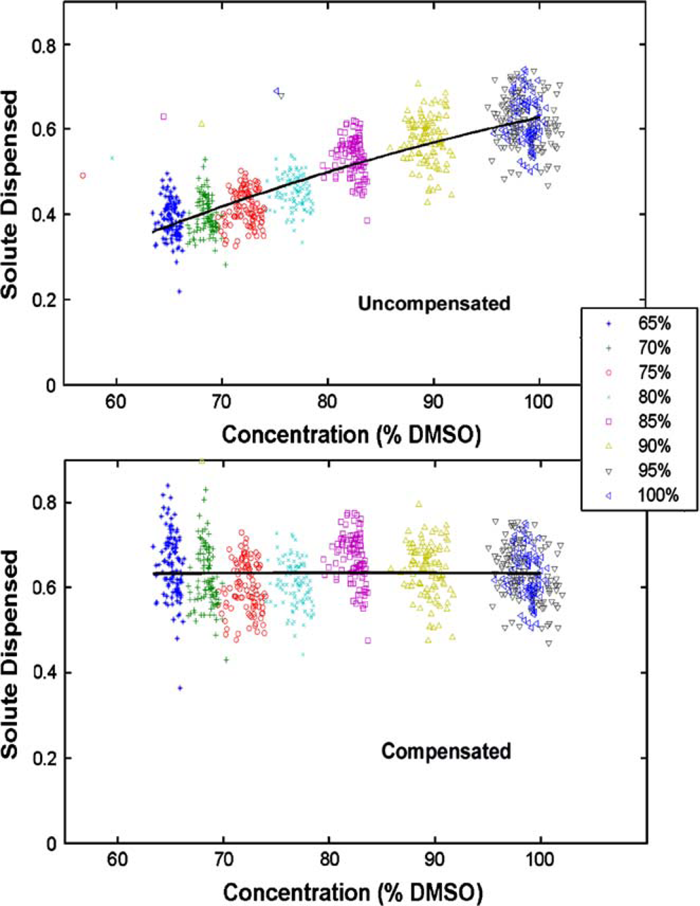

However, by knowing the estimated DMSO concentration by volume, the corresponding volume ejected may be increased to eject the same amount of DMSO for each drop. The bottom plot in Figure 10 shows the effect of using this compensation method.

This method for DMSO concentration compensation has been incorporated into the EDC acoustic technology platform. If compensation is desired, the tool may be configured to measure the DMSO concentration and compensate by changing volume ejected to assure uniform solute dispensing.

Appendix a – the Dynamic Model

A classic damped harmonic oscillator may be used to describe the primary mode of oscillation of the stimulated surface. This is described with the following equation:

$$f\left(t\right)=Tx\left(t\right)+v\dot{x}\left(t\right)+m\ddot{x}\left(t\right)$$

(7)

where f(t) is the applied force function, x, $\dot{x}$ and ẍ are the displacement, first derivative with respect to time, and the second derivative with respect to time, T is the spring constant or in this case the surface tension, v is the viscous damping constant, and m is the effective mass of the fluid.

In this case, the surface is initially at rest and it is stimulated with an impulse function. Therefore, the differential equation may be solved using the Laplace transform method where the Laplace transform of Eq. (7) yields:

$$m{s}^{2}x\left(s\right)+vsx\left(s\right)+Tx\left(s\right)=f\left(s\right)$$

(8)

and solving for x(s)

$$x\left(s\right)=\frac{f\left(s\right)}{m}\frac{1}{{\left(s+v/2m\right)}^2\hspace{0.17em}+\hspace{0.17em}\left(T/M-v^2/4m^2\right)}$$

(9)

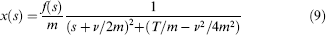
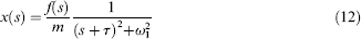
Traditionally, at this point a substitution of ω₁ and τ is made as follows:

$${\omega }_1^2\equiv T/m-v^2/4m^2$$

(10)

$$\tau =v/2m$$

(11)

which simplifies Eq. (9) to

$$x\left(s\right)=\frac{f\left(s\right)}{m}\frac{1}{{\left(s+\tau \right)}^2+{\omega }_1^2}$$

(12)

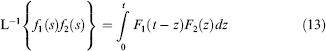
This Inverse Laplace Transform is solved by using the convolution theorem

$${\text{L}}^{-1}\left\{f_1\left(s\right)f_2\left(s\right)\right\}=\underset{0}{\overset{t}{\int }}{F}_1\left(t-z\right)F_2\left(z\right)dz$$

(13)

The impulse function f(t) = Pδ(t), where P is the momentum transferred and δ(t) is the Dirac delta function. By using the known Laplace Transform:

$$\text{L}\left\{{\text{e}}^{at}\sin \left(kt\right)\right\}=\frac{k}{{\left(s-a\right)}^2+k^2}$$

(14)

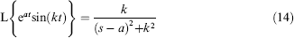
Eq. (13) becomes

$${\text{L}}^{-1}\left\{\frac{1}{m{\omega }_1}f\left(s\right)\frac{{\omega }_1}{{\left(s+\tau \right)}^2+{\omega }_1^2}\right\}=\frac{P}{m{\omega }_1}\underset{0}{\overset{t}{\int }}\delta \left(t-z\right){\text{e}}^{-\tau z}\sin \left({\omega }_{1}z\right)dz$$

(15)

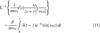
Therefore

$$x\left(t\right)=\frac{P}{m{\omega }_1}{\text{e}}^{-\tau t}\sin \left({\omega }_{1}t\right)$$

(16)

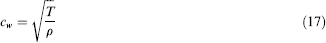
The model used in this analysis also depends on the boundary condition of the surface of the fluid or a vibrating circular membrane. The general solution to this problem has been worked out by Kinsler and Frey in “Fundamentals of Acoustics”. ⁶ In our analysis, we are only concerned with the specific case where the center of the membrane is stimulated and the membrane is allowed to vibrate while the displacement of the center is measured over time. In this case, the solution of the problem is simplified and based on the fundamental properties of the membrane, namely the surface density ρ, the surface tension T, and the radius of the membrane a. The velocity of transverse surface waves is given by

$$c_w=\sqrt{\frac{T}{\rho }}$$

(17)

And, based on the solutions of the membrane oscillation equation, the frequency of the oscillation at the center of the membrane is determined to be

$${\omega }_1=2.40483\frac{c_w}{a}$$

(18)

where the constant is derived from the first root of the zeroth order Bessel function J₀(x). It is quite clear from this relationship that the frequency is dependent on the radius of the well at the surface of the fluid, which varies from 0.85 mm at the top of the well to 0.68 mm at the bottom of the well.