
Abstract
Examining the influence of culture on personality and its unbiased assessment is the main subject of cross–cultural personality research. Recent large–scale studies exploring personality differences across cultures share substantial methodological and psychometric shortcomings that render it difficult to differentiate between method and trait variance. One prominent example is the implicit assumption of cross–cultural measurement invariance in personality questionnaires. In the rare instances where measurement invariance across cultures was tested, scalar measurement invariance—which is required for unbiased mean–level comparisons of personality traits—did not hold. In this article, we present an item sampling procedure, ant colony optimization, which can be used to select item sets that satisfy multiple psychometric requirements including model fit, reliability, and measurement invariance. We constructed short scales of the IPIP–NEO–300 for a group of countries that are culturally similar (USA, Australia, Canada, and UK) as well as a group of countries with distinct cultures (USA, India, Singapore, and Sweden). In addition to examining factor mean differences across countries, we provide recommendations for cross–cultural research in general. From a methodological perspective, we demonstrate ant colony optimization's versatility and flexibility as an item sampling procedure to derive measurement invariant scales for cross–cultural research. © 2020 The Authors. European Journal of Personality published by John Wiley & Sons Ltd on behalf of European Association of Personality Psychology
Keywords
In the last two decades, several large–scale studies have compared personality assessment across cultures to examine the extent to which culture exerts an influence on an individual's personality (Allik et al., 2017; Bartram, 2013; Kajonius & Mac Giolla, 2017; McCrae, 2001; Schmitt et al., 2007). These studies’ findings indicated, for example, a similar structure of personality across cultures (Allik, Realo, & McCrae, 2013; McCrae, 2001) and primarily small differences between cultures in personality factors (Allik et al., 2017), which can to some extent be grouped geographically and culturally (e.g., Schmitt et al., 2007). For example, in Allik and McCrae (2004), European and American countries had higher values in Openness and Extraversion, but lower values for Agreeableness compared with Asian and African samples. Cross–cultural personality studies usually rely on mean levels of self–reported personality traits measured with translated instruments across several culturally dissimilar countries. Thus, researchers often implicitly assume that personality instruments measure the same or a sufficiently similar construct across cultures (e.g., McCrae, 2002; Schmitt et al., 2007).
More recent studies have begun to test this assumption of cross–cultural measurement invariance (MI) in a more thorough, confirmatory way. They have concluded that none of the most common personality measures achieve scalar cross–cultural invariance (Church et al., 2011; Nye, Roberts, Saucier, & Zhou, 2008; Thielmann et al., 2019). Scalar MI refers to the same assignment of items to factors with equal item loadings and intercepts across cultural groups. It is a prerequisite for an unbiased comparison of factor means across cultures. For example, a lack of scalar invariance was uncovered in the revised version of the NEO Personality Inventory (Costa & McCrae, 1992)—one of the most frequently used instruments to assess the Big Five personality factors (i.e., Agreeableness, Conscientiousness, Extraversion, Neuroticism, and Openness)—and in the HEXACO Personality Inventory–Revised (Lee & Ashton, 2004), which is based on a six–factor model of personality. A lack of MI represents one of the central methodological problems in cross–cultural personality research and calls the robustness of previous study results into question. Solutions to this issue have already been proposed in the literature, usually taking the form of some type of less strict invariance testing (Cieciuch, Davidov, Algesheimer, & Schmidt, 2018; Muthén & Asparouhov, 2018; Steenkamp & Baumgartner, 1998) that conceals the non–invariance of personality instruments in cross–cultural contexts. Another way of overcoming this issue is to develop measures that are measurement invariant, thus enabling meaningful cross–cultural personality comparisons.
In this paper, we present an item sampling technique for compiling cross–cultural measurement invariant measures. We begin by summarizing the results of previous studies on personality across cultures with a special focus on MI test results. Subsequently, we discuss the methodological prerequisites for studying personality across countries. Finally, we present an item sampling procedure, ant colony optimization (ACO), that can derive invariant short scales and exemplify its versatility by sampling invariant items for two different groups of countries: one characterized by cultural similarity and the other by cultural dissimilarity. In doing so, we show to what extent cultural differences affect the possibility of finding invariant item sets.
Cross–cultural studies of personality differences
Since 1990, the number of studies in the field of cross–cultural personality research has grown substantially (Boer, Hanke, & He, 2018). Table 1 provides an overview of some of the most prominent cross–cultural personality studies conducted in the last two decades. We only included studies comparing five– or six–factor personality models across several countries using self–reports; therefore, it is not an exhaustive list of all cross–cultural personality studies. Overall, the presented studies are heterogeneous in terms of countries, languages, and measurement instruments.
Overview of cross–cultural personality studies
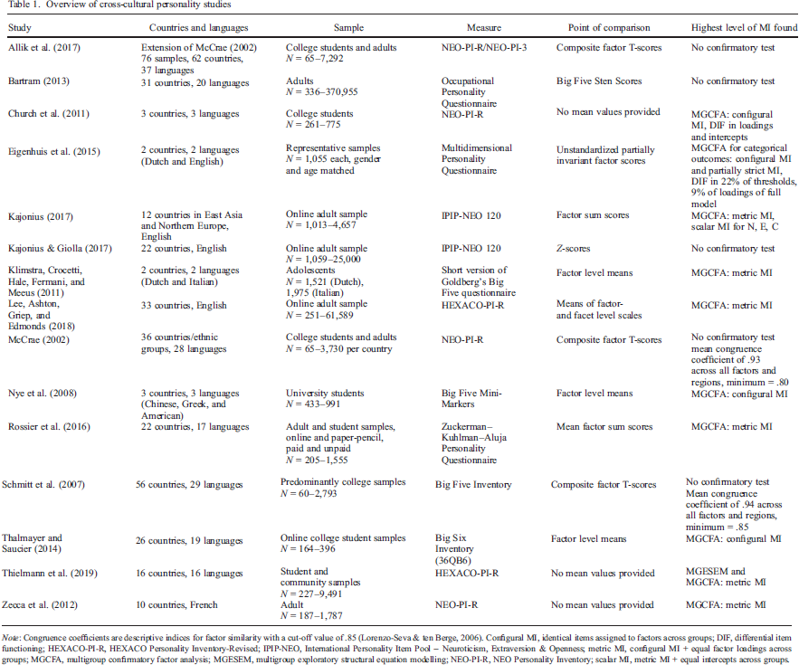
Note: Congruence coefficients are descriptive indices for factor similarity with a cut–off value of .85 (Lorenzo–Seva & ten Berge, 2006). Configural MI, identical items assigned to factors across groups; DIF, differential item functioning; HEXACO–PI–R, HEXACO Personality Inventory–Revised; IPIP–NEO, International Personality Item Pool – Neuroticism, Extraversion & Openness; metric MI, configural MI + equal factor loadings across groups; MGCFA, multigroup confirmatory factor analysis; MGESEM, multigroup exploratory structural equation modelling; NEO–PI–R, NEO Personality Inventory; scalar MI, metric MI + equal intercepts across groups.
On the one hand, this diversity in methods and approaches is positive because, in a sense of a conceptual replication, the results do not rely on the specific instantiation (e.g., based on either five factors or six factors of personality). On the other hand, it limits a direct comparison of countries across studies, as any differences found can be either methodological or substantial. Below, we critically discuss some methodological and content–related aspects that these studies have in common.
First, the cross–cultural samples used within these studies vary widely in terms of size, age, gender distribution, and data collection method (with the exception of Eigenhuis, Kamphuis, & Noordhof, 2015). Particularly in the large–scale studies (Allik et al., 2017; Bartram, 2013; McCrae, 2002; Schmitt et al., 2007), the samples were often rather small convenience samples (e.g., 60 college students for Cyprus in Schmitt et al., 2007) that were already available and published (i.e., not collected with the intention of using them for cross–cultural comparisons). Thus, the samples often cannot be considered representative for the respective countries.
Second, all of the presented studies comparing personality across countries use composite or sum scores (again, except for Eigenhuis et al., 2015). That is, in most studies, it is implied that the scale score provides an adequate representation of the underlying personality trait without properly testing this assumption. In the studies in which the respective instrument's model fit was tested in a confirmatory way, the models rarely yielded good fit, which is in line with previous statements on the model fit of personality instruments in general (Hopwood & Donnellan, 2010). Accordingly, the aggregated manifest scores cannot be meaningfully used and interpreted, as they violate the assumption of unidimensionality for a specific personality trait. Because personality inventories often show no simple structure, less stricter approaches such as Exploratory Structural Equation Modelling (ESEM; Asparouhov & Muthén, 2009) have been proposed as a potential remedy to this problem. ESEM combines characteristics of Confirmatory Factor Analysis and Exploratory Factor Analysis, that is, allowing for cross–loadings while also reassessing model fit indices (Marsh et al., 2009).
Third, we want to highlight an aspect that affects all studies listed in Table 1 and is arguably the most problematic—the lack of scalar MI across cultures. MI addresses the question of ‘whether or not, under different conditions of observing and studying phenomena, measurement operations yield measures of the same attribute’ (Horn & McArdle, 1992, p. 117). Therefore, cross–cultural comparison always hinges on MI. To answer the question whether different cultures or countries are similar or dissimilar with respect to underlying latent traits, it must be ensured that the results are not affected by the measurement itself. The studies presented in Table 1 can be divided into two groups in this respect: in one third of the studies, universal applicability for mean comparisons was either not tested or justified using congruence coefficients of loading patterns derived from exploratory factor analysis (Allik et al., 2017; Bartram, 2013; Kajonius & Giolla, 2017; McCrae, 2002; Schmitt et al., 2007). However, comparing loading patterns across groups is not a confirmatory test of MI. In the remaining studies, MI was tested with the most commonly used procedure for testing measurement equivalence across groups, Multi–Group Confirmatory Factor Analysis (MGCFA). Scalar MI did not hold for any of the personality measures. In order to demonstrate the implications of this result, we briefly introduce the procedure for testing MI in a MGCFA framework and explain the importance of scalar MI for the comparison of means.
Measurement invariance in cross–cultural personality research
In MGCFA, MI is tested in several steps involving increasingly restrictive constraints on measurement parameters (e.g., Meredith, 1993; Milfont & Fischer, 2010; Vandenberg & Lance, 2000). Usually, MI testing encompasses four consecutive steps (Schroeders & Gnambs, 2020, but see also Wicherts & Dolan, 2010). In the first step, configural MI, only the way items are assigned to factors identical across groups. Second, in metric MI, factor loadings are constrained to be equal, while other measurement parameters are freely estimated. This level of MI allows for the comparison of bivariate relations, such as factor correlations, correlations to covariates, and factor variances, between groups. In the third step, scalar MI, intercepts are additionally constrained to be equal across groups, which is a prerequisite for unbiased comparisons of factor means. Finally, in strict MI, the residual item variances must also be equal across groups, which allows for a comparison of manifest scale scores across groups. In summary, different levels of MI permit different types of cross–cultural comparisons. In cross–cultural personality assessment, the goal is often to compare means, which requires scalar MI. If this level is not achieved, any group differences found may also be attributed to measurement bias. Consequently, measurement per fiat, that is simply stating that an aggregate score is unidimensional and comparable across different contexts, is insufficient. Ways to circumvent full scalar MI have been suggested, such as partial scalar MI (e.g., Steenkamp & Baumgartner, 1998), alignment with an optimized simplicity function (for an example application, see Muthén & Asparouhov, 2018), and approximate MI (e.g., Cieciuch et al., 2018).
While we acknowledge that methods such as partial MI can reduce bias in latent variable modelling under certain conditions, they do not solve the underlying problem of non–invariant indicators. Simulations convincingly demonstrate the detrimental effect of a lack of MI on the validity of mean comparisons (Steinmetz, 2013), especially when sum scores are used (i.e., assuming strict MI)—which is often the case in cross–cultural personality comparisons. Comparisons of factor means can also be distorted by items that lack scalar MI. A simulation study by Chen (2008) demonstrated that cross–culturally variant item loadings and intercepts can lead to pseudo group differences due to an overestimation of the mean in the group with higher loadings or intercepts and an underestimation in the other group. In addition, partial MI (i.e., allowing some variant parameters to freely vary between groups) is also a conceptual issue: letting item parameters vary freely across groups conceals the fact that the measurement model is not identical in terms of its mean and variance–covariance structure. In many cases, the results would be different had the construct been measured with an invariant instrument (Chen, 2008). Therefore, despite these alternative modelling suggestions, group comparisons with full scalar invariant item sets should be the primary objective to avoid bias.
Consequently, based on these methodological considerations and the fact that none of the most common personality measures have been found to be cross–culturally (scalar) invariant (see Table 1), previous mean comparisons reported in the literature on personality across cultures must be treated with caution. Some scholars have already acknowledged this point and did not list or compare countries’ means (e.g., Church et al., 2011; Zecca et al., 2012). In case studies that did report mean–level differences in personality factors between countries, they were often small and unsystematic. Accordingly, the cross–country personality similarities hypothesis (Kajonius & Mac Giolla, 2017) postulates that personality similarities between countries outweigh differences. However, due to the non–invariant measurement instruments used in cross–cultural personality studies so far, statements about personality differences across cultures can only be trusted to a limited extent. This raises the question of how the mean values of personality factors or facets actually vary across cultures and whether these differences are consistently greater in comparisons between culturally dissimilar countries. To answer these questions, a scalar invariant personality questionnaire is needed that is suitable for comparing even culturally dissimilar countries.
Thus, we next discuss potential causes of MI across cultures. van de Vijver and Tanzer (2004) differentiated among three types of bias in cross–cultural assessment: item bias, method bias, and construct bias. Examples of item bias are culture–specific interpretations of item content or a poorly translated questionnaire that changes its meaning. For instance, in one study, an incorrect translation of the word ‘crime’ into Danish probably resulted in unexpectedly high levels of tolerance towards criminal immigrants among Danish participants (Davidov, Meuleman, Cieciuch, Schmidt, & Billiet, 2014). A second possible cause for a lack of MI could be that participants’ response behaviour differs across cultures (Johnson, Kulesa, Cho, & Shavitt, 2005; Wong, Rindfleisch, & Burroughs, 2003), which represents an aspect of method bias. For example, acquiescence—the tendency to agree to an item regardless of its content—has been found to vary between cultures (Smith et al., 2016). Further method bias could result from the fact that participants in one country are more familiar with self–reports than others. While these problems can be addressed with straightforward countermeasures (see, e.g., Hambleton, 2005, for translation guidelines), the following other sources of bias might be more complicated to overcome. Construct bias caused by poor sampling of relevant behaviour, different definitions of constructs across cultures, and differential appropriates of the behaviours associated with the construct can also influence the way people respond to items. Different display rules across cultures are a good example for a mixture of item and construct bias, as individual items referring to exhibiting overt behaviour in public might only be a good indicator for extraversion in certain cultures. For example, extraverted people in the USA express positive emotions (e.g., happiness or surprise) more often, whereas this behaviour is discouraged in Japan. Instead, extraverted people in Japan show more assertive behaviour (Ekman & Friesen, 1969; Safdar et al., 2009).
As a result, comparing dissimilar cultures using a single measure developed in a Western culture has been criticized, because it imposes a Western factor structure while neglecting behaviour that might be important for understanding the other culture (Heine & Buchtel, 2009). Within these fixed sets of personality items, some items may be cross–culturally applicable, some may be culturally invariant for specific countries, and some may only be suitable for the country where the measure was initially developed. Without a comprehensive theory on how culture or situations influence personality, it is impossible to flag problematic items prior to testing. Rather than accepting these issues and relaxing model constraints to allow for cross–cultural differences at the item level that cannot be explained by the underlying latent constructs, we propose a different approach: we understand existing personality questionnaires as an item pool from which to sample items under certain constraints. Below, we present a data–driven approach to sampling cross–culturally invariant items to enable unbiased cultural personality comparisons between given sets of countries.
Ant colony optimization
Sampling items from a larger item pool to compile an invariant, reliable, and sound short scale can be viewed as a combinatorial problem. The larger the item pool and the more criteria that should be considered in the construction, the more difficult it is to find a solution manually. ACO is a meta–heuristic optimization procedure that can find optimal or close–to–optimal solutions within a proportion of model estimations by mimicking the behaviour applied by ants in search of food (Dorigo & Stützle, 2010). In a nutshell, ants communicate by leaving pheromones on their way towards a potential food source, thus attracting subsequent ants. This optimization principle is flexible and has been applied to the selection of items or the development of short scales in different contexts (e.g., Janssen, Schultze, & Grotsch, 2017; Leite, Huang, & Marcoulides, 2008; Olaru, Schroeders, Hartung, & Wilhelm, 2019; Olaru, Schroeders, Wilhelm, & Ostendorf, 2018; Olaru, Witthöft, & Wilhelm, 2015; Schroeders, Wilhelm, & Olaru, 2016a, 2016b).
Ant colony optimization is an iterative algorithm. In the first iteration, several item sets are randomly selected from the item pool and evaluated based on the specified optimization criterion (e.g., MI across countries). It is also possible to combine several criteria that should be considered in evaluating the item sets (e.g., MI and reliability of the scale). Each item set used to estimate the model corresponds to an ant searching for a route. The items comprising the best model in the initial iteration will have a higher probability of being selected (= virtual pheromone levels) in subsequent iterations. Similar to the way pheromones accumulate faster on shorter routes, being part of the best solution in one iteration increases an item's selection probability in subsequent iterations. Across several iterations, a close–to–optimal or optimal item solution given the user–specified optimization criteria can be found. There are several parameters that influence the breadth and depth of the search behaviour (Olaru et al., 2019; Schultze & Eid, 2018). For example, the number of virtual ‘ants’ within each iteration can be defined, with more ‘ants’ resulting in a longer but also more precise search, as more models are compared in each iteration. Or to reduce the pheromone levels of items that were only selected in early iterations when the selection probability is close to chance, an evaporation parameter can be specified that reduces all items’ pheromone levels after each iteration (Leite et al., 2008). Evaporation ensures that the pheromone level of inferior items is constantly reduced.
Sampling items via ACO has several advantages in comparison with traditional item selection procedures such as selecting items with the highest item–total correlation (e.g., Leite et al., 2008; Olaru et al., 2018; Schultze & Eid, 2018): First, ACO is much more computationally efficient than testing all possible models (in our study,
The present study
To allow for meaningful cross–cultural personality comparisons, we used ACO to compile item sets that provide unidimensional, reliable, and cross–culturally measurement invariant assessments of the personality factors. We derived a measurement invariant short scale from a larger set of 300 personality items, namely, the IPIP–NEO 300 (Goldberg, 1999), across two sets of countries—a similar set of the so–called Western world (i.e., USA, UK, Australia, and Canada) and a culturally dissimilar mix of countries (i.e., USA, India, Sweden, and Singapore). Countries were defined as culturally similar versus dissimilar based on their scores on Hofstede's cultural dimensions (Hofstede, Hofstede, & Minkov, 2010), which have shown significant connections with personality in previous cross–cultural studies (e.g., Hofstede & McCrae, 2004). On the dimension individualism, for example, values for the culturally dissimilar countries were much more divers (Singapore = 20, India = 48, Sweden = 71, and USA = 91) on a scale of 1 (collectivism) to 100 (individualism) than values for the similar countries (all between 80 and 91). We chose to include the USA sample in both groups because it has often been used as a reference group in cross–cultural research (Allik et al., 2017; Schmitt et al., 2007). With the present article, we pursue three major goals. First, we test the flexibility and versatility of ACO by creating measurement invariant short versions of the IPIP–NEO for groups of culturally similar and dissimilar countries. Second, we use the resulting short versions of the IPIP–NEO to examine potential cross–cultural differences in personality. For example, we scrutinize differences in the factor means across culturally similar versus dissimilar countries. Third, from a methodological perspective, we show how researchers could potentially use customizable item selection procedures to create measurement invariant short scales for their own purposes to avoid measurement bias.
Method
Sample and measure
We reanalyzed an open data set (https://osf.io/wxvth/) collected online (http://www.personal.psu.edu/∼j5j/IPIP/) in which personality was measured with the IPIP–NEO 300 (Goldberg, 1999). The IPIP–NEO 300 measures the Big Five—Agreeableness, Conscientiousness, Extraversion, Neuroticism, and Openness, each of which consists of six facets measured by 10 items each. Participants had to indicate their agreement with the different statements on a 5–point scale (1 = very inaccurate, 2 = moderately inaccurate, 3 = neither accurate nor inaccurate, 4 = moderately accurate, and 5 = very accurate).
The data have already been examined for duplicate participation, missing values per person, and obviously inattentive or aberrant repetitive response patterns (Johnson, 2014). In this process, 26,848 cases, or 8.03% of the original 334,161, were removed from the data set (for the exact cleaning procedure, see Johnson, 2005). Besides age, gender, and the country to which ‘one feels most likely to belong’, no demographic variables were available. The data cover the period from 2001 to 2011 and a total of 307,313 participants from 235 differently named regions, with cases such as Vatican (N = 2) and Vatican Cit [sic] (N = 6) artificially increasing this number. Among the 212,625 participants, the USA makes up a clear majority (69%).
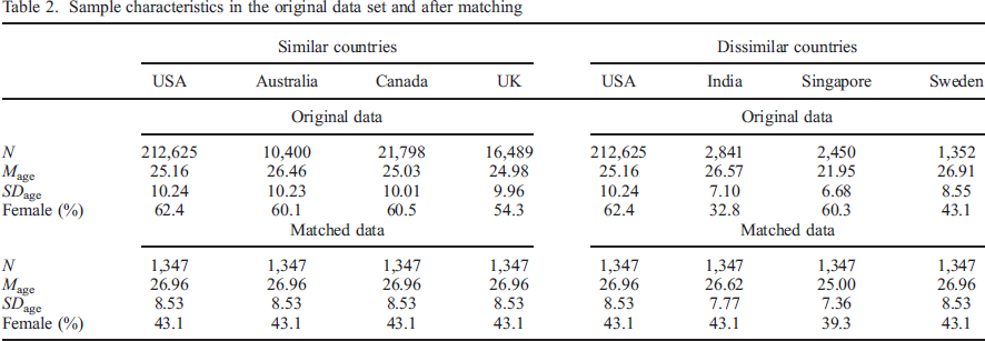
Because unequal sample size and composition across country groups can lead to biased results in MI testing (Yoon & Lai, 2018), we matched the samples of our selected countries by means of propensity score matching (Caliendo & Kopeinig, 2008). Matching aims to reduce the person sampling bias by creating samples that are comparable on observed covariates (in our case, age and gender). We only included participants who were between 14 and 70 years old at the time of the survey. Sweden had the smallest N within our set of selected countries, so it served as a reference group. Propensity score matching was conducted with the nearest neighbour method included in the R package matchit 3.0.2 (Ho, Imai, King, & Stuart, 2011) in order to generate comparable samples in terms of sample size, age, and gender for all seven countries (see Table 2). Nearest neighbour matching selects the closest control match for each individual in the reference group. Thus, all subsequent analyses were carried out with samples of 1347 participants per country (matched to the age and gender distribution of Sweden).
Sample characteristics in the original data set and after matching
Statistical analyses
Model specification
To account for the hierarchical nature of personality, we specified a bifactor model with a general factor reflecting one of the Big Five traits, consisting of all 18 selected items, and six personality facets, consisting of three items each (see Figure 1). The general factor and the six facets were all uncorrelated. There are two substantial arguments for choosing a bifactor rather than a higher–order model: first, the testing procedure for scalar invariant higher–order models is overly strict (Chen, Sousa, & West, 2005), because both the measurement and structural parts of the model must be constrained to be equal across groups, including the first–order and second–order factor loadings. However, constraining the second–order factor loadings to equality in order to meaningfully compare the means of the traits is equivalent to constraining the factor correlations in a correlated facet model. We argue that these parameters constitute structural parameters rather than measurement parameters and should be freely estimated (see also Olaru et al., 2018). Second, in the scalar invariant higher–order model, the facet level means must be constrained to equality (Chen, West, & Sousa, 2006). Thus, such a model does not allow for comparing the means on the facet level. In contrast, a scalar invariant bifactor model allows for comparing the freely estimated means across countries (Schroeders & Jansen, 2020). Thus, bifactor modelling provides a significant advantage over a higher–order model when the goal is to conduct unbiased comparisons of facet and factor means. Moreover, assuming equal means on the facet level seems overly restrictive and does not reflect the research literature or the existing empirical data. In sum, the separation of interindividual differences into general and domain–specific variance in a bifactor model seems advantageous because it provides a framework for analysing to what extent heterogenous items reflect general factor (trait) or more conceptually narrow subcomponents (facets).
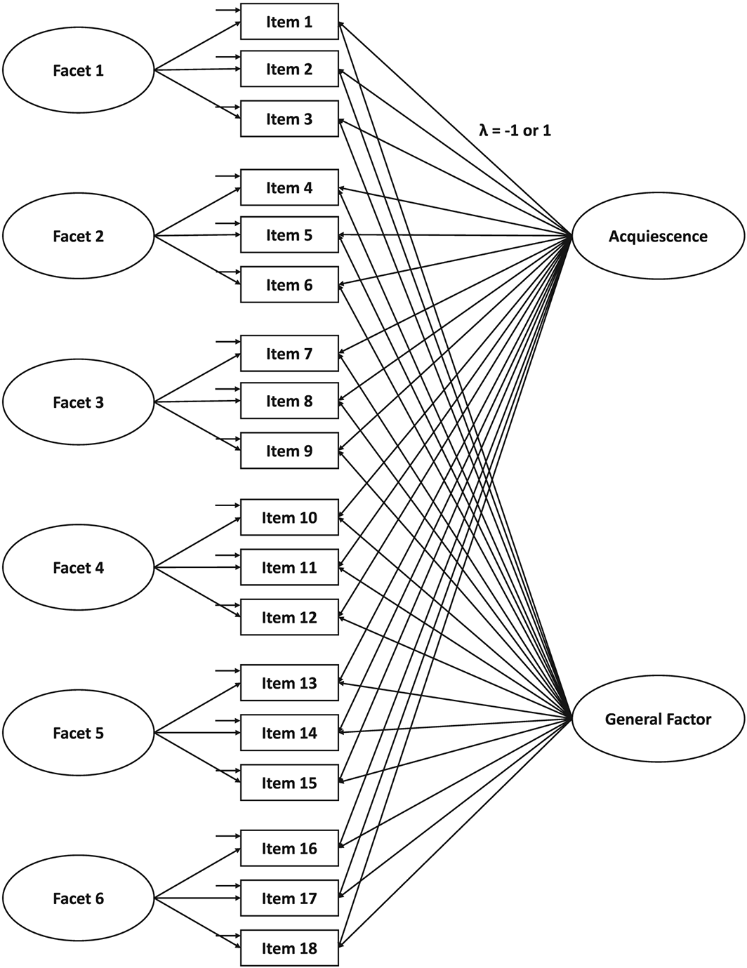
Example bifactor model for one Big Five factor.
To account for response style effects, we specified an acquiescence factor across all facets, that is, factor loadings were fixed to 1 for all positively keyed items and −1 for all negatively keyed items (Billiet & McClendon, 2000; Ferrando & Lorenzo–Seva, 2010). Because acquiescence is presumed to vary across cultures (Smith, 2004), we specifically incorporated this source of systematic variance (bias) into the measurement models. Simulation studies showed that ordinal data with at least five response categories can be treated as continuous when not heavily skewed (Beauducel & Herzberg, 2006; Rhemtulla, Brosseau–Liard, & Savalei, 2012). Therefore, parameter estimations were based on a maximum likelihood procedure with robust estimation of standard errors. All models were estimated using the full information maximum likelihood method, which is a model–based approach for handling missing data (Schafer & Graham, 2002). Compared with other missing data handling procedures, full information maximum likelihood allows for more precise parameter estimation and retains statistical power because no observations are deleted (Enders, 2010). All analyses were conducted in R 3.4.4 (R Development Core Team, 2018); the R package lavaan 0.5–23 was used for the SEM (Rosseel, 2012).
Item selection via ant colony optimization
We selected three out of 10 items per facet, resulting in 18 items per IPIP–NEO factor. This yielded a total of almost 300 billion possible item combinations per factor. Thus, we used an item sampling procedure, ACO, to simultaneously optimize four item selection criteria. First, as suggested by Hu and Bentler (1999), we evaluated model fit with a combination of an absolute fit index, the root mean square error of approximation (RMSEA), and an incremental fit index, the comparative fit index (CFI), with CFI > .95 and RMSEA < .05 considered an indication of a good model fit. These two criteria were equally weighted in the pheromone function. The second criterion concerns MI between countries. MI across groups can be tested with a MGCFA comprising increasingly restrictive measurement models (for a more detailed description, see Schroeders & Gnambs, 2020). Thus, we estimated three models for each item set: the configural measurement model, the metric measurement model (with equality constraints on the factor loadings), and the scalar measurement model (with equality constraints on the factor loadings and the item intercepts). A cut–off of ΔCFI > .01 between consecutive models (i.e., configural vs metric and metric vs scalar) was taken to indicate a significant deterioration in model fit caused by the additionally introduced constraints (Cheung & Rensvold, 2002).
The third criterion refers to the reliability of the general factor and the facets averaged across groups. We used the McDonald (1999) ω as a measure of reliability, because in contrast to Cronbach's α, it does not require an essentially tau–equivalent measurement model with equal factor loadings of all items (Zinbarg, Revelle, Yovel, & Li, 2005). It only requires a tau–congeneric model in which factor loadings are allowed to vary, which is a less strict and more realistic assumption. For the general factor, we considered ω > .70 as sufficiently high, whereas the minimum was ω > .30 for the facets because the factor saturation of nested factors is considerably smaller (Brunner, Nagy, & Wilhelm, 2012). Differently put, the specific factors in a bifactor model represent the residualized common variance among the items of a specific facet. As a fourth criterion, we aimed to select an equal number of positively and negatively keyed items. Thus, nine negatively keyed items out of 18 per personality factor were defined as optimal, with the highest pheromone level. The more unequal this ratio became, the stronger the decrease in pheromone level along a normal distribution. All four criteria were logit–transformed to differentiate more strongly between values close to the respective cut–off (e.g., Schroeders et al., 2016b) and then summed to form the algorithm's overall optimization function. However, we assigned the scalar MI criterion twice as much weight as the other criteria due to its central role in unbiased comparisons. For an overview of the exact equations, please see Appendix A.
To exclude problematic models such as Heywood cases (Kolenikov & Bollen, 2012), we included a check for estimation issues (i.e., errors within lavaan). Such problematic models were not considered in the optimization process, or their pheromones were set to zero. Other possible modelling issues, such as residual correlations, cross–loadings, or low factor loadings, were adequately addressed by the criteria used (model fit and reliability). Because ACO is a probabilistic rather than a deterministic approach and often finds several different solutions across several runs that are similarly psychometrically sound, we carried out a total of five ACO runs, each with different seeds. The syntax and the results of all ACO iterations are available at https://osf.io/ds7j5/files/.
Results
In this section, we first present the model fit for the configural measurement models with 60 items for each factor of the IPIP–NEO (i.e., bifactor model with six specific factors), which serve as a reference point for comparisons with the short versions. We then discuss the results of the item selection via ACO with respect to the optimization criteria, namely, (a) model fit, (b) MI across countries, (c) reliability, and (d) ratio of negatively and positively keyed items.
In the group of culturally similar countries, the models for each Big Five factor in the long version yielded insufficient fit. CFI ranged from .771 for Agreeableness to .858 for Neuroticism. RMSEA ranged from .051 for Openness to .057 for Extraversion/Agreeableness. In the group of culturally dissimilar countries, model fit was also inadequate: the CFI ranged from .768 for Agreeableness and .863 for Neuroticism, while the RMSEA ranged from .048 for Neuroticism to .054 for Extraversion. Because the fit values indicated insufficient model fit for the full scale, we elected not to calculate reliability estimates or test for MI.
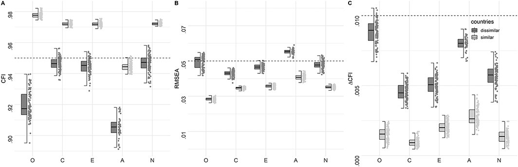
The following results refer to all short versions derived by means of ACO that meet the metric MI criterion. Figure 2 presents model fit (CFI and RMSEA) and scalar MI (∆CFI) distributions across all models estimated during the ACO search procedure. Due to ACO's fit function, the distributions are skewed towards the positive pole of the indicators (e.g., towards higher CFI). Nonetheless, the distributions of the two model fit indices (CFI and RMSEA) and the scalar MI criterion (∆CFI) substantially differ for the two groups of countries. Specifically, there were more good fitting models for the group of similar countries compared with the group of dissimilar countries (see Figure 2A and B). While almost all solutions for the culturally similar countries were scalar invariant (98.42%), this was only true of 31.85% of the solutions for the dissimilar countries (see Figure 2C). The distribution of ∆CFI illustrates that scalar MI is not a particularly strong problem for the culturally similar countries in our study and that optimizing scalar MI is much more relevant for culturally dissimilar countries. For the similar countries, 39.66% of solutions satisfied all three criteria (i.e., RMSEA, CFI, and ∆CFI). In contrast, for the dissimilar countries, only 0.29% of solutions satisfied the criteria. It is therefore not only more difficult to find invariant solutions for dissimilar countries—the pool of solutions that represent a good compromise between the different criteria is also much more limited.
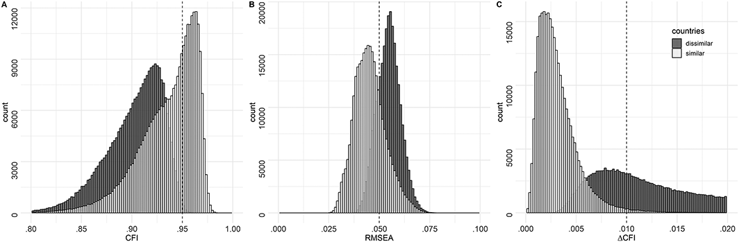
Distributions of CFI, RMSEA, and ΔCFI between the metric and scalar measurement models for all item sets. The gray dashed line in panels (A) and (B) indicates the criterion for good model fit (CFI > .95 and RMSEA < .05, Hu & Bentler, 1999). The gray dashed line in panel (C) denotes the commonly used cut–off for measurement invariance of .01 by Cheung and Rensvold (2002).
Next, we focus on the 100 best solutions across the five ACO runs (defined by the highest pheromone values) for each factor. 1 We decided to evaluate the best 100 instead of the single best solution in order to examine and visualize the variability in the results set. Figure 3A and B presents the CFI and RMSEA of the best 100 solutions. Compared with the long version, the model fit of the short versions was substantially better in both country groups. This improvement in model fit cannot solely be attributed to the reduced number of items, because there were also many models with insufficient model fit (see Figure 2). In the group of culturally similar countries, the model fit for all item sets except those for Agreeableness reached the specified cut–off. Although model fit also improved in the culturally dissimilar group, lower model fit values were achieved. For the Agreeableness and Openness factors, no item set reached CFI > .95 and RMSEA < .05. In general, good model fits were obtained for Conscientiousness, Extraversion, and Neuroticism in both groups of countries.
Distributions of indices of model fit and measurement invariance of the 100 best ACO solutions. (A) comparative fit index (CFI); (B) root mean square error of approximation (RMSEA); (C) CFI of metric versus scalar measurement models (ΔCFI). The boxplot reflects the interquartile range, the solid line represents the median, and the whiskers represent minimum/maximum values within 1.5 times the interquartile range. The gray dashed line in panels (A) and (B) indicates the criterion for good model fit (CFI > .95 and RMSEA < .05, Hu & Bentler, 1999). The gray dashed line in panel (C) denotes the commonly used cut–off for measurement invariance of .01 by Cheung and Rensvold (2002).
For both groups, the best 100 ACO solutions all met the scalar MI criterion, with the exception of five models for Openness in the group of dissimilar countries (see Figure 3C). Also, in this group, decreases in model fit were higher, with Agreeableness and Openness, the most problematic factors, corroborating the aforementioned result. Note that as more criteria are optimized and evaluated, the potential pool of adequate solutions becomes smaller. As such, there is a trade–off between the number of optimization criteria included in the optimization function and the potential number of adequate solutions.
For the general factor, the average McDonald's ω of the 100 best solutions did not differ much between the culturally similar countries and the culturally dissimilar countries (see Figure 4). Sufficient factor saturation (ω > .70) was obtained for all best item sets. The factor saturation distributions for the best 100 ACO results for the personality facets can be found in Figures S1–S5 at https://osf.io/fnbqj/. There was also no clear pattern as to which group of countries had higher factor saturation regarding the facets. In general, there was notable variation in the facets’ factor saturation within the best 100 solutions for both groups. However, all item sets reached the chosen cut–off on the facet level (ω > .30).
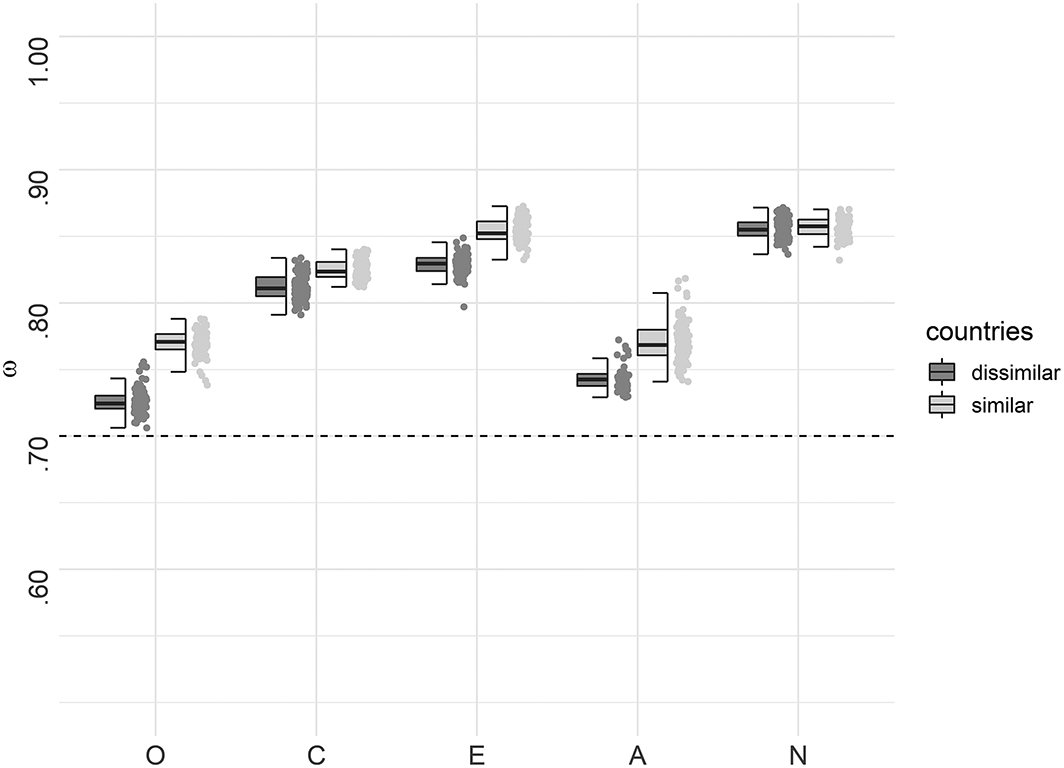
McDonald's ω for the 100 best ACO solutions for the general factors. The boxplot reflects the interquartile range, the solid line represents the median, and the whiskers represent minimum/maximum values within 1.5 times the interquartile range. The gray dashed line represents the criterion of ω = .70.
As a further criterion in the optimization function, we balanced out negatively and positively keyed items, as is recommended to control for potential response bias (Soto & John, 2018). In the group of culturally similar countries, ACO selected nine negatively keyed items out of 18 items per factor in 498 of the best 500 solutions for all five personality factors. In the group of dissimilar countries, some unbalanced item combinations were selected, because more compromises between the criteria had to be made (e.g., MI and a balance of positively and negatively keyed items). The deviation from the optimal number of positive/negative items was small, as the number of negatively keyed items ranged between 8 and 11 and the majority of solutions (70%) contained an equal number of negatively and positively keyed items here as well.
In summary, ACO managed to compile item sets with an appropriate model fit, factor saturation, and balanced number of positively versus negatively keyed items that are also cross–culturally scalar invariant, making it possible to meaningfully compare factor means across countries. It must be pointed out, however, that for all criteria except factor saturation, ACO was able to find more suitable solutions for the group of culturally similar countries than for the group of dissimilar countries. As the distributions of model fit illustrate (Figure 2), model fit was higher on average for the similar countries from the start, meaning that this criterion was met in many models even without optimization. In the dissimilar country group, however, finding acceptable solutions for Openness and Agreeableness was not always possible. Finding optimal solutions becomes generally more difficult as the number of criteria increases, particularly if one of these criteria significantly reduces the pool of potential solutions from the onset. In the present study, there had to be at least 18 scalar measurement invariant items per personality factor in the data. Incorporating multiple criteria such as MI, model fit, reliability, and a balanced number of positively and negatively keyed items restricts the item selection even more. In sum, item selection can compensate for deviations (e.g., measurement variant items) to a certain degree, but it is not a panacea for finding solutions that are not possible in a given data set.
Personality differences across countries
In the following, we report mean–level differences between the examined countries. We plotted standardized factor means for the trait factor and the six facets for the 100 best solutions that were scalar measurement invariant for both groups. Hereby, we show not only the average differences in means between countries but also the distributions of means within each individual country. Figures 5 and 6 depict the distributions of the five general factors for both groups of countries, with the USA as a reference point (i.e., factor mean fixed to zero). Mean differences for all 30 personality facets of the IPIP–NEO can be found in Figures S6–S15 at https://osf.io/fnbqj/.
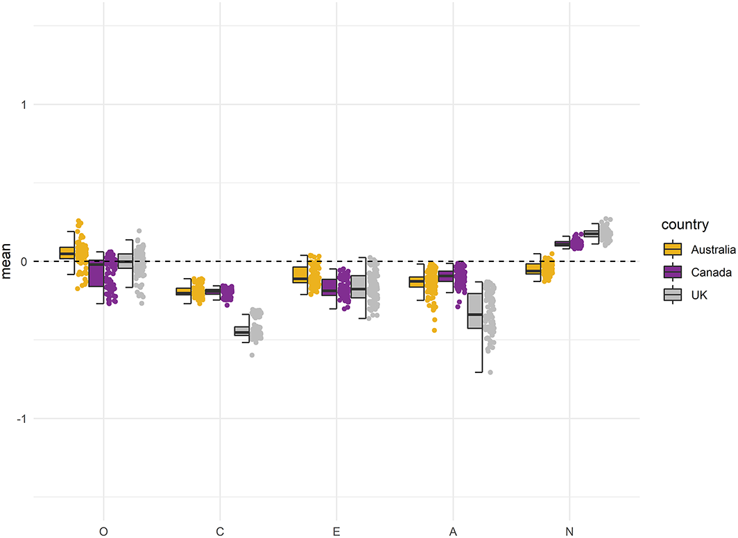
Standardized means of the general factors for the culturally similar countries. The boxplot reflects the interquartile range, the solid line represents the median, and the whiskers represent minimum/maximum values within 1.5 times the interquartile range. The mean of the reference group (US) is fixed to 0.
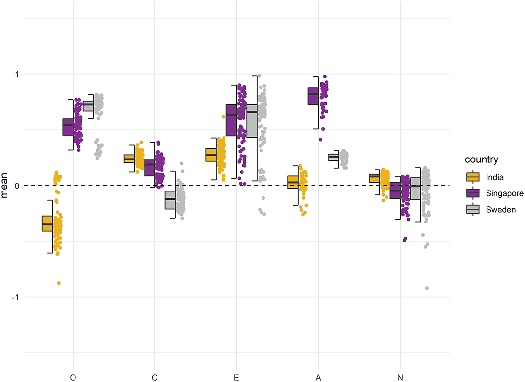
Standardized means of the general factors for the culturally dissimilar countries. The boxplot reflects the interquartile range, the solid line represents the median, and the whiskers represent minimum/maximum values within 1.5 times the interquartile range. The mean of the reference group (US) is fixed to 0.
As the primary goal of this article is to demonstrate how ACO can create culturally measurement invariant short forms, we will only discuss some general trends in the results set. The standardized mean differences between the four countries were larger on average within the group of culturally dissimilar countries. In the group of similar countries, the absolute mean differences varied mostly between 0 and 0.50, representing a nil to medium effect size according to Cohen (1988). For Extraversion (see Figure 5), for example, the absolute differences in the similar group were less than 0.40. In the group of dissimilar countries, most mean differences for Conscientiousness and Neuroticism were also nil to medium sized (see Figure 6). Larger mean differences were found for Agreeableness, Openness, and Extraversion. For example, Singapore had mean values on these factors more than 0.50 higher than those of the USA. In this context, however, it is important to note the large variation in factor means over the best solutions.
Thus, we conclude that item selection played a substantial role in most cases and led to differences in the countries’ means that were often as large as, or even larger than, the average mean differences between countries. For example, depending on the selected item set for the Extraversion factor, one could conclude that Swedish people are on average either very extraverted, with a standardized mean 0.90 higher than US citizens or that both groups are essentially alike. Consequently, item sampling effects are not trivial when interpreting country comparisons, and using a fixed set of items across countries is by no means a gold standard approach. In our study, mean differences in the personality facets exhibited a very similar pattern as those for the general factors in terms of magnitude: differences between countries and variability between item sets were larger on average in the group of dissimilar countries. However, there were no clear pattern for the resulting differences across countries within the individual factors. For example, Sweden had the lowest values of Orderliness within the group of dissimilar countries but had the highest for Self–Efficacy (facets of Conscientiousness, see Figure S9). Typically, cross–cultural studies report mean–level differences at the Big Five level, while there is also substantial variation at the facet level.
Discussion
The lack of scalar MI is a common problem in cross–cultural personality studies (see Table 1) that renders mean value comparisons potentially biased (e.g., Church et al., 2011; Nye et al., 2008; Thielmann et al., 2019). Even if one theoretically assumes that personality is universal across cultures, this does not imply that a given measure must be empirically invariant across cultures. Researchers who compare personality across cultural groups should test whether the personality measure used is indeed suitable for the intended comparison. According to the Standards for Educational and Psychological Testing (AERA, APA, & NCME, 2014), test fairness refers to the fact that test scores should have the same meaning for all participants independent of other, non–related participant characteristics such as age, sex, or country. For example, comparing the mean structure of measures that are not at least scalar invariant is biased, and decisions derived on this basis may disadvantage certain groups of people solely due to their group membership (see Wicherts & Dolan, 2010, for an example concerning IQ test scores among minorities). One way to avoid such consequences would be to only use the items of a test that are at least scalar invariant across groups, which could be achieved with item sampling procedures such as ACO.
In this study, we aimed to compile culturally invariant and psychometric sound short scales of the IPIP–NEO 300 that can be used for unbiased personality assessment across countries. In ACO, several criteria can be incorporated in the item selection process simultaneously (i.e., model fit, MI, factor saturation, and ratio of negatively and positively keyed items). Importantly, it was possible to create such scales for two different groups of countries—Western countries (culturally similar) and a more diverse set of countries (culturally dissimilar). Thus, item sampling procedures such as ACO represent a promising method for studying differences across countries. Although it was possible to compile scalar invariant short scales, there were differences in the efficiency of the optimization between the two groups. The results suggest that it is unproblematic to achieve scalar MI for culturally similar countries, while there are significantly fewer invariant item subsets among culturally dissimilar countries. However, we think a larger item pool can compensate for this: for example, the Synthetic Aperture Personality Assessment project is currently collecting data with 92 openly available personality measures and several thousand items, thus providing an ample item pool (Condon & Revelle, 2015). On the one hand, because participants complete not all items but a random selection of them, such approaches come at the cost of massive missingness. On the other hand, by abandoning the assumption of fixed measurement instruments, such projects can take on the idea of sampling items rather neatly: with enough participants, these projects may be able to provide further insight into what constitutes a trait or facet.
In our study, we found mainly moderate differences in personality traits across the country samples, which were larger on average within the group of culturally dissimilar countries. It has been a common practice to calculate sum or mean scores for the five or six respective personality factors and compare them across countries (e.g., Allik et al., 2017; McCrae, 2002; Schmitt et al., 2007). However, the non–uniform rankings of the individual countries across different individual facets of each factor in our study indicate that it is advisable to consider differences at lower levels and not merely aggregate facets into factor scores. The specified bifactor model is particularly useful for this purpose, because—if scalar MI holds—it enables unbiased mean comparisons of both the personality facets and the general factors.
Limitations and future research
It is a recurring criticism that shortening a scale also reduces measurement precision on the individual level (Mellenbergh, 1996), reliability on the group level (e.g., Kruyen, Emons, & Sijtsma, 2013), and construct coverage (Schroeders et al., 2016a). This is a truism but also that coefficients of reliability and construct validity of unabbreviated versions are biased if the measurement model does not hold to the empirical data. In this respect, item selection procedures can help by simultaneously incorporating model fit, reliability, construct coverage, and other quantifiable criteria into the optimization function (Schroeders et al., 2016a). For example, it is possible to add item characteristics such as content and linguistic features to ensure that they are sufficiently covered in the shorter scale. However, doing so requires a larger number of items. Nevertheless, the potential caveats of shortened scales are not trivial, and selecting the most appropriate items for a specific context is always a compromise between maximizing different criteria (e.g., MI vs construct coverage).
A potential limitation of creating short scales with ACO is that it is a data–driven procedure that optimizes the model based on the specific criteria and sample. Hence, it must be ensured that the results do not only hold for a specific instantiation of items. Item sets that result in an invariant model with good fit values in one sample may therefore be unsuitable for another (e.g., different countries). Researchers who aim to create short scales with the help of meta–heuristics should be aware of this fact and should not assume that the results will generalize. One way of quantifying the robustness of the item selection results across different samples is to cross–validate them using an independent validation sample (Olaru et al., 2019), as is also often recommended in the machine learning literature (Yarkoni & Westfall, 2017). In the present article, however, we employed another way of evaluating heterogeneity in the results: because it is a probabilistic rather than a deterministic approach (Olaru et al., 2019), ACO often finds several psychometrically sound solutions across several runs, which could lead to conflicting conclusions (e.g., regarding the ranking of different countries according to their means). In our study, for example, there was considerable variability within the 100 best ACO solutions. In particular, with regard to the comparisons of facets, for which country means were relatively similar, the differences between solutions within a given country were larger than average differences between countries. Thus, if only one ACO run is performed, the analysis conducted using this single item set could be strongly dependent on the respective selection (capitalizing on chance). Therefore, it is recommended to run the metaheuristic procedure several times to examine variability across different results sets.
In summary, results always depend on the specific items or scales used. This is especially true for constructs such as personality, even beyond the application context of item sampling itself, because the items making up different personality assessment measures represent nothing more than different subsets of all possible items. Therefore, the item set–specific variability of results is not only an ACO or personality issue; it applies to any item set (i.e., measurement instrument) with a potentially large item pool (i.e., item universe). Thus, the dependence on item sampling used should always be kept in mind when interpreting study results. This statement is discouraging if the ultimate goal is to develop a universal instrument suitable for all contexts. However, researchers can also view this as an opportunity to deviate from given item sets because published measures do not constitute an irrefutable item set.
Recent studies have proposed a different take on personality assessment than reflective modelling, namely, that the items themselves capture important aspects of personality and yield incremental predictive validity over and above the facets or factors (McCrae, 2015; Mõttus et al., 2019; Mõttus, Kandler, Bleidorn, Riemann, & McCrae, 2017; Seeboth & Mõttus, 2018). This ‘residual’ variance has been labelled personality nuances (McCrae, 2015; Mõttus et al., 2017). From this perspective, item selection and consequently exclusion could be seen as problematic at first glance. However, the perspectives of item sampling and personality nuances have much in common: feature selection, which is part of many machine learning techniques (Chandrashekar & Sahin, 2014), is in a way analogous to item selection via ACO because it selects the most predictive items for a given set of outcomes. For example, Seeboth and Mõttus (2018) used elastic net regression to examine the criterion–related validity of items within the 50–item Big Five personality questionnaire (Goldberg, 1999) and showed that models based on item uniqueness explained 30% more variance on average in 40 different outcomes (e.g., income, body mass index, or Internet use) than models based on the Big Five. Note, however, that modelling item uniqueness comes at the cost of abandoning the idea of a reflective model which assumes that all meaningful variance in the indicators is caused by latent factors. Moreover, machine learning predictions often lack theoretical foundation.
Measurement invariance—two sides of the same coin
Apart from using measurement invariant item sets for comparing facet and factor means, it may also be worthwhile to investigate sources of non–invariance. Non–invariant items may be especially interesting with respect to cultural differences, as they might serve as indications of divergent response behaviour to certain questions and their underlying causes (for a classification of possible sources of cross–cultural bias, see van de Vijver & Tanzer, 2004). Church et al. (2011) termed this phenomenon DIF paradox, because researchers on the one hand seek to exclude items that are non–invariant in order to conduct meaningful comparisons, yet on the other hand, the excluded items may convey important personality nuances for understanding cultural differences. In other words, there is a trade–off between optimizing comparability across cultures (MI) and sensitivity within each country (cross–cultural variability). The two approaches do not contradict but rather complement one another. In summary, we think that cross–cultural differences in nuances—or differential item functioning, in technical terms—represent two sides of the same coin: in cases in which mean differences are of particular interest, scalar measurement invariant instruments should be used for comparisons, with ACO as a tool to compile such item sets. If researchers are interested in studying cultural differences in more detail, non–invariant items might be more informative. To conclude, in cross–cultural personality research, we must take issues of MI more seriously than in the past and must reflect on the methodological and trait–related causes of measurement variance.
Footnotes
Appendix
All four criteria were logit–transformed to differentiate more strongly between values close to the respective cut–off and to scale the value range between 0 and 1 (e.g., Schroeders et al., 2016a, 2016b). CFI > .95 and RMSEA < .05 were considered as indications of a good model fit, so both were averaged for the first criterion of the pheromone function as follows
The second criterion was scalar measurement invariance across countries. ΔCFI reflects the absolute difference in CFI between the configural and metric as well as metric and scalar models; the chosen cut–off for both comparisons was 0.01 (Cheung & Rensvold, 2002):
As a third criterion, a minimum factor saturation of McDonald's ω (McDonald, 1999) > .70 for the general factor and > .30 for the specific facets was considered sufficient:
ω was calculated as the relation of the squared sum of the factor loadings to the sum of the residuals for each country for all the general factors and facets as the 2 in the following equation are exponents, I changed it backfollows:
The four values of the countries within each group were then averaged. Because all six facets of a factor were considered in the selection process simultaneously, the cut–off for the specific facets reflects whether the lowest ω of the six facets averaged across four countries reached the criterion of .30.
For the fourth criterion, the balance of positively and negatively keyed items, a function was defined which reaches an optimum of 1 at an equal number of negatively and positively keyed items and decreases with a normal distribution as this ratio becomes more unequal:
In the pheromone function, the four criteria were summarized and maximized over the course of the iterations. Measurement invariance was assigned twice as much weight as the other three criteria: