
Abstract
In this paper, we propose a novel simultaneous registration and fusion approach for tracking. This method is based on a recursive Variational Bayesian (RVB) algorithm, which is the online variant of the Variational Bayesian (VB) approach. Under the Bayesian framework, the states and parameters are recursively estimated. It is shown by simulation that the proposed RVB method has better estimation performance than the conventional approach.
1. Introduction
Sensor fusion is an essential component for a sensor network to improve the overall system performance [1]. It is a method of integrating signals from multiple sources into a single signal or piece of information. Considering the fact that multiple sources have their own coordinate systems, it is necessary to transform the local measurements into a common coordinate and estimate the sensor bias to perform alignment. The fusion centre is then applied to estimate the target states. Therefore, the fusion process relies on an accurate registration of sensors. The lack of proper registration will cause poor performance in the fusion process.
In order to obtain more information, intelligent vehicles should register and fuse numerous data from multi-sensors, such as cameras, lidars and radars. For instance, in a multi-radar multi-target system, each radar range and azimuth bias can cause significant errors in the target location. Therefore, many sensor registration algorithms have been proposed in the literature, such as the least squares (LS) method [2] and the maximum likelihood estimator method [3–4].
Some methods have been proposed to address the problem of registration and fusion simultaneously, which can be performed at the measurement level or track level. In [5], a joint sensor registration and fusion approach at the measurement level was proposed using an expectation-maximization (EM) algorithm. In [6], by using a pseudo-measurement approach, simultaneous registration and fusion was performed at the track level.
However, such studies focus on the batch algorithm, which estimates the parameter based on all data. This method is impractical for real-time processing. Therefore, many online algorithms have been proposed to address this problem. The traditional method is that the sensor bias is included in the augmented state equations, and then the Kalman filter, extended Kalman filter (EKF) or unscented Kalman filter (UKF) is used to estimate the augmented states’ systems. In [7], Okello, et al. formulated the joint registration and fusion at the track level as a Bayesian estimation problem, and proposed the extended Kalman filter (EKF) by augmenting the state vector with sensor bias. In [8], the augmented Kalman filter was proposed to perform the sensor registration.
In this paper, we propose a novel method to recursively perform simultaneous registration and fusion at the measurement level. The RVB [9] is the recursive variant of Variational Bayesian (VB) inference, which is an approximation to the exact Bayesian inference, where the true posterior is approximated using a simpler distribution. VB has low computational costs in comparison with the sampling methods, such as Markov Chain Monte Carlo (MCMC). It has widespread use in machine learning, signal processing and many other fields, such as the state space model [10, 11], time series [12, 13], Mixture Models [14], filter [15–17], image [18–20], communication [21, 22], speech recognition [23] and graphical models [24, 25].
The problem of joint sensor registration and fusion at the measurement level has been seen as the estimation of parameters on the Bayesian framework. Combining them with the expectation-maximization (EM) algorithm, states and parameters are formulated via Recursive Variational Bayesian Expectation Maximization (RVBEM). Compared with the augmented Kalman filter [8], the proposed method has a better performance.
The paper is organized as follows. The problem of simultaneous registration and fusion is formulated in Section 2. In Section 3, the RVBEM for simultaneous registration and fusion are developed in detail. Computer simulations are shown in Section 4. Finally, some concluding remarks are given in Section 5.
2. Problem Formulation
In tracking, it is assumed that the target state evolves according to a linear, discrete time model of the form:

where

where
The state is driven by an initial state x0, which is assumed to be a Gaussian process with mean
Then, we choose the standard conjugate priors for the model. Firstly, the prior of the initial state x0 and the sensor bias is defined as:

The Gaussian density is defined as:
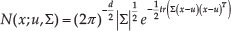
where u and Σ is the mean and precision of the normal distributed, respectively, and d is the number of the dimension of x.
The prior over the measurement noise precision matrix R, which is assumed to be diagonal, has Gamma prior:

where m is the number of dimension of R,
The Gamma density is defined as:

where a and b is the shape and inverse scale of the gamma distributed, respectively.
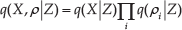
Therefore, the overall joint density as:

where X={x1, x2…… xT} is the hidden state and Z={z1, z2……., zT} denotes the data.
3. RVBEM for Simultaneous Registration and Fusion Recursively
Based on the Bayes’ theorem:

where
The log of marginal likelihood can be written as:

where

where F is the free energy:

and KL is the Kullback-Liebler divergence between the approximate posterior
and the true posterior

The goal of VB is to minimize the KL-divergence. However, the KL-divergence cannot be directly minimized, because the true posterior
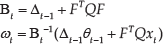
where

where

and

where
This leads to a set of coupled update rules. Iterated application of these leads to the desired maximization. The resulting VB algorithm follows an EM update procedure. In the Variational Bayesian expectation (VBE)-step, the variational posteriors over hidden variables are calculated. In the Variational Bayesian Maximization (VBM)-step, the variational posteriors over parameters are updated. Each step is guaranteed to increase the lower bound of the marginal likelihood. We choose every size of the batch from a single data point. The RVBE and RVBM are iterated until convergence, which occurs rapidly. After convergence, the prior of parameters for the next batch is set as the current posterior.
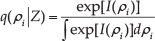
The optimal components of the approximation posterior are defined as:

Note that the form of the posterior distribution is the same as in the prior distribution. The prior distributions are chosen to conjugate with the likelihood [26]. In what follows, the states and parameters of distributions are updated.
E-step
In this step, we update the distribution of hidden variables using the variational forward algorithm [11].
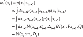
Forward pass: the predictive density:
where
Set:
Then the predictive density
Therefore, the mean and covariance of the predictive density are defined as:
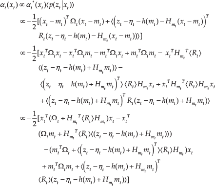
Forward pass: the updated density:
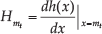
Taylor-expand h(x) at the predictive estimate of state:
where H is the Jacobian
Then, we get the mean and covariance of the updated density:


M-step
The detailed derivations of the updated parameters are given in this step.
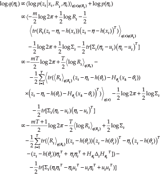
Update for η
The form of log posterior density can be rewritten as:
Comparing the coefficients with equations (29) and (30), we get:
So: The prior of the next batch is set as:
Update for R:
The form of the log posterior density can be rewritten as:
Comparing the coefficients with equations (33) and (34), we get:
Therefore, The prior of the next batch is set as:


In [26], Beal et al. pointed out that the underfitting may occur in this online algorithm, which is due to excessive self-pruning of the parameters by the VB algorithm. An annealing variant of the RVBEM algorithm by making use of an inverse temperature parameter is proposed. We adopt the following update for the RVBM step instead of eqs. (31)–(35).


The pseudo-code of RVBEM is given as follows:
Initialize
For t=1,2……T (observations)
2.1 RVBEM
RVB-E step: Update the parameters of the approximate distributions’ hidden states using the variational forward algorithm.
RVB-M step: Update the parameters of the approximate posteriors over the parameter as in (37) and (38).
2.2 After convergence, the prior of the next batch is set to the current posterior as in (32) and (36).
4. Simulations
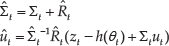
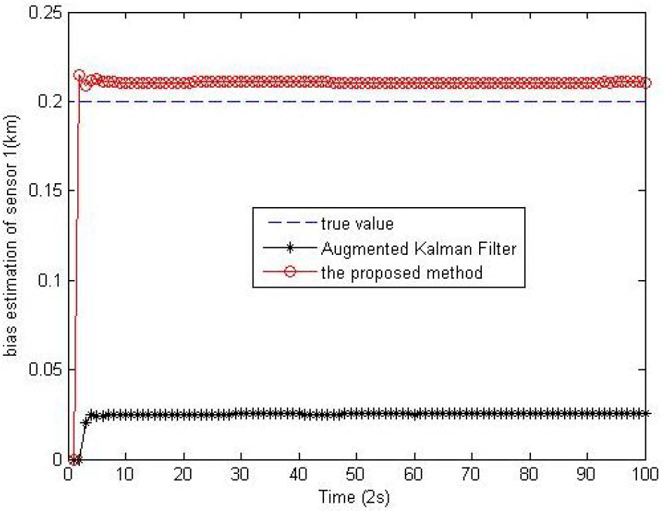
In this section, we used the proposed algorithm to estimate registration and fusion simultaneously online via computer simulations. Two radars are used to track one target with a constant velocity motion. The positions of Sensor 1 and Sensor 2 are at (0 km, 0 km) and (200 km, 0km), respectively. The target speed is 0.5 km per second at the x-coordinate and 0 km per second at the y-coordinate. The initial position of the target is at (50 km, 30 km). The sensors measure the target every two seconds. The registration error of Sensor 1 is (0.2 km, −0.15 rad), and the registration error of Sensor 2 is (−0.2 km, 0.15 rad). The process noise covariance is set as diag(0.0001km2, 0.0001rad2, 0.0001km2, 0.0001rad2). The number of time instants is 150.
Estimation of the range bias at Sensor 1

Estimation of the azimuth bias at Sensor 1
In practice, we set the priors of gamma distribution as
Case 1. We choose the measurement noise covariance to be set equal to diag(0.0005km2, 0.0005rad2). To illustrate the registration performance of the proposed method, Figures 1 to 4 show the convergence of the estimated registration parameters.
Estimation of the range bias at Sensor 2

Estimation of the azimuth bias at Sensor 2

MSE in the position estimation of x
We evaluate the performance using mean squared error (MSE) over 1000 runs for the estimated target state. Figures 5 to 6 show the MSE of the estimate of the target using the two methods. It is observed that the estimation performance of the proposed method is better than that of the Augmented Kalman Filter.

MSE in the position estimation of y
The computation is performed on a desktop computer with a Core 2 DUO 2.53 GHz and 2GB RAM. For a single run, the RVB requires 0.188s and the Augmented Kalman filter needs 0.093s. By augmenting the state vector in the augmented Kalman filter, the memory requirement of the augmented Kalman filter is more expensive than that of the RVB.

Estimation of the variance at Sensor 1 inthe range
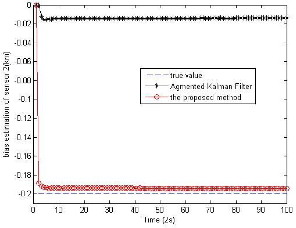
Case 2. In order to illustrate the performance of estimating the non-stationary time-varying parameters, we set the measurement noise first, which has variance diag(0.0005km2, 0.0005rad2); at time t=1000, the variance is then quickly increased to diag(0.002km2, 0.002rad2) and then t=2000 is again quickly decreased back to diag(0.0005km2, 0.0005rad2). In addition, the number of measurements taken is 4000. The other parameters are the same as in Case 1. The results of the estimates of non-stationary measurement noise variance are shown in Figures 7 to 10. It is observed that the estimates of the proposed method follow the true variance fairly well.

Estimation of the variance at Sensor 1 in azimuth
Estimation of the variance at Sensor 2 in range

Estimation of the variance at Sensor 2 in azimuth azimuth
5. Conclusion
In this paper, the problem of online joint sensor registration and fusion were seen in terms of estimating parameters of the Bayesian framework. We proposed using a RVBEM algorithm to perform it simultaneously. The posterior distributions of the states and parameters were presented in detail. Our proposed method shows better performance when compared to the augmented Kalman filter, which was validated using the computer simulation. Future work will plan to extend the algorithm to cope with the problem of joint sensor registration and fusion when the target number is unknown and variable.
Footnotes
6. Acknowledgements
This work is jointly supported by the Zhejiang Open Foundation of the Most Important Subjects, the Research Funds of Chongqing Science and Technology Commission (Grant No.cstc2013jcyjA40042) and by the National Natural Science Foundation of China (Grant No. 61301033).