Sage Journals: Discover world-class research

Abstract

The purpose of this article is to verify the possibility of using artificial neural networks (ANN) in business management processes, primarily in the area of supply chain management. The author has designed several neural network models featuring different architectures to optimize the level of the company's inventory. The results of the research show that ANN can be used for managing a company's order cycle and lead to reduced levels of goods purchased and storage costs. Optimal neural networks show suitable results for subsequent prediction of the amount of items to be ordered and for achieving reduced inventory purchase and keeping costs down.

Keywords

Lot-sizing Problem Inventory Management Artificial Neural Network

1. Introduction

In today's highly competitive economic environment, characterized by low profit margins, high requirements for product quality and short delivery times, commercial companies are forced to take every opportunity to optimize their business processes.

Inventory management is considered one of the most important functions of manufacturing and trading companies and can have an impact on the overall performance of the business. Very often it is necessary to consider the trade-off between the cost of storage and the high cost of losses resulting from low levels of inventory and an inability to satisfy the customer. The best solution is effective inventory management, which ensures a good level of services without excessively large levels of stock that disproportionately increase storage costs.

The purpose of this article is to examine suitable methods of artificial neural networks (ANN) and their application in business processes, especially in inventory management. It discusses the construction of an ANN model. The designed model can be used for inventory level optimization to improve the ordering system and inventory management. The methods used in this paper are primarily ANN and ANN-based modelling. Sales data of a wholesale trade fastening-materials company are used for analysis and prediction.

The aim is to detect whether ANN methods are suitable tools to enhance a company's ordering system and, if so, in what architecture.

The theory of inventory management is probably one of the most researched areas of manufacture and trade. Although almost all major manufacturing and trading companies and many small- and medium-sized companies try to apply scientific methods to manage their inventory better, the use of these methods is often limited to a few basic tools [1].

The paper introduces the efficacy and applicability of ANN modelling and forecasting in the context of supply chain management, especially inventory management. Within the research, several types of neural networks are created. Each neural network is then verified; based on this, the most effective architecture of the neural network is determined.

The task of inventory management models is to appropriately regulate levels of inventory, mostly with regard to the cost of storage and ordering. So far, however, a universally suitable model for inventory management has not been developed, so in each specific situation, the optimal solution for the inventory model must be found as a derivative of existing models.

2. Literature Review

The first mathematical model for inventory management, the Economic Order Quantity (EOQ) model, was introduced in 1913 by Ford W. Harris [2]. It was designed for the purpose of production planning. The EOQ is a one-product deterministic dynamic model and is essentially very simple: periodically replenished inventory with a constant level of supply. The aim of the EOQ model is to find the size of production or purchase supply to make the company's activities the most economically advantageous. It is necessary to balance acquisition costs with the cost of storage.

The EOQ model is often modified for different methods of entering required input data, e.g., if there is a need to respect the rebate (quantity discounts depending on the volume of the ordered quantity in the supply) or to consider other initial assumptions of the model.

The study of miscellaneous model situations, focusing on simulating conditions, searching for results and optimal solutions are among the most important contemporary trends [3, 4]. Over the years, countless studies have looked for the optimum result for inventory management or similar issues from supply chain management [5, 6].

Many inventory models have been constructed with different input assumptions [7 –15] within the supply chain.

Ioana et al. [16] presented a new concept for fuzzy logic in economic processes. Zhang [17] investigated the estimated technical efficiency score's sensitivity through different methods including the stochastic distance function frontier.

ANN models have been successfully used to solve the demand forecasting and production scheduling problem. Gaafar and Choueiki [18] applied a neural network model to a lot-sizing problem as a part of material requirements planning (MRP) for the case of deterministic time-varying demand.

A paper introduced by Megala and Jawahar [19] deals with a dynamic lot-sizing problem including capacity constraint and discount price structure. Two meta-heuristics – genetic algorithm and Hopfield neural network – are established for the dynamic lot-sizing problem. In recent years many other global publications have dealt with the lot-sizing problem, which has recently been solved by heuristics [20 –25].

An ANN structure was also used by Hamzaçebi [26] and compared with traditional statistical methods. The results from the modelled ANN utilized for time-series forecasting proved that the proposed ANN model comes with significantly lower prediction error than other methods.

Research presented by Hachicha [27] also utilized an ANN and worked with the lot-sizing problem in supply chains by applying a metamodelling simulation. The supply chain, which is also a subject of Hachicha's research, is handled in a make-to-order environment (no possibility of keeping stock and limited production capacity). The model is designed for multi-product, multi-stage and multi-location production planning with capacity constraints and stochastic parameters such as lot arrival orders, transit time, set-up time, processing time and so on. In practical applications the results confirm the effectiveness, flexibility and usability of the ANN method.

Paul and Azaeem [28] developed another ANN-based model that determines the optimum level of a finished goods inventory. Inputs to this model are product demand, setup, holding, and material costs, where data originated from a manufacturing industry. The results indicated that the model can be used for a finished goods inventory level forecasting in response to the model input parameters. In general, the constructed model can be applied for finished goods inventory optimization in any manufacturing enterprise.

In research by He [29], a fast convergent Back Propagation (BP) neural network model for inventory level prediction is introduced. The paper predicts the inventory level of an automotive parts company by applying the improved BP neural network model. The results of the research show that the improved algorithm not only exceeds the standard algorithm but also outperforms some of the other improved BP algorithms.

The mentioned scientific publications often deal with the application of neural networks in determining the size of supplies for manufacturing companies. Some of the authors admit insufficient consideration of the need to minimize the costs associated with delivering the goods. Here possibilities for further research appear, while making use of neural networks to determine the size of the supply in the trading business as well as the relevant costs.

3. ANN Model

The aim of the research is to use ANN methods to design the ordering cycle of a company. This paper presents an ANN model that can be used to optimize inventory levels and thereby improve inventory management and the ordering system of the company.

Input, output and test data were provided by an existing company: a wholesale retailer of fastening materials. The company buys from an Asian supplier and, as a part of a supply chain, has to account for a replenishment delivery time of approximately 60 working days from the date of the order. The collected data are from the company's recent history and cover one month's sales of the type of the company's goods with highest turnover.

The model is constructed for deterministic demand and non-deteriorating goods. Backlogging is not permitted.

The objective function of the ANN model can be demonstrated as:

O Q = f (I D a c t, I D 3, I D 33, I I, I P, I T)

(1)

As input parameters of the model, the following variables are used:

the current demand, IDact≥0,

the demand in the next three months, ID3≥0,

the demand in the three months after the three-month ordering cycle, ID33≥0,

the current inventory level, II≥0,

the purchasing cost per unit of item, IP>0,

the procurement cost per unit of item, IT>0.

As output data, the amount ordered was designated OQ>0.

MS Office Excel was used for data analysis, pre-processing and standardization; MathWorks MATLAB Neural Network Tool was used for neural network forecasting.

In this study, an ANN model was developed to determine the optimal amount of goods to be ordered to optimize the current quantity of goods in stock. To construct the ANN model, the selection of input and output parameters is crucial. For this model, six of the most important factors, which influence decision-making for the ordered quantity, were chosen as input variables. They include the current demand (monthly), demand in the next three months, demand in the three months after the three-month ordering cycle, the current value of stock, the purchase price per unit of goods, and procurement cost per unit of goods. As a unit of goods, 1,000 pieces of specific goods are taken. The model's output parameter is then the optimal quantity purchased. The representation of inputs and outputs can be seen in Figure 1.

Figure 1.

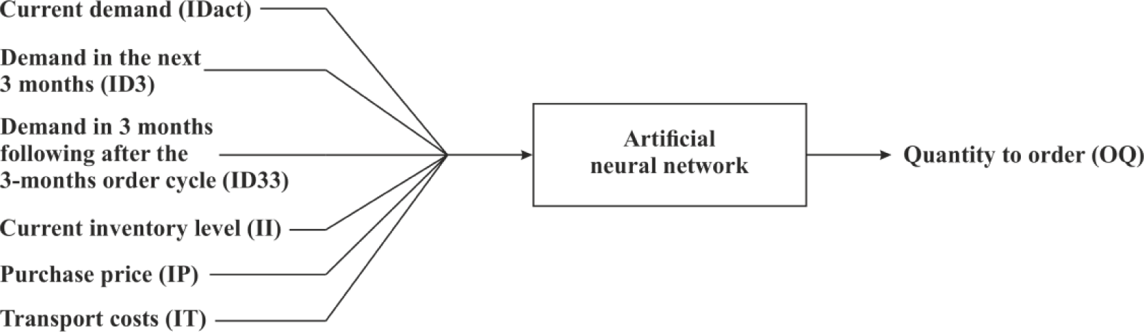
Neural network's inputs and output diagram

For the design and construction of the neural network model, the following steps need to be taken: the collection of input, output and sample datasets, and designing, training and verification of the neural network. After obtaining the sample dataset, the data are pre-processed to input-output patterns. Input and output data are standardized to values from interval <0;1> to obtain a consistent result using ANN.

Outputs, i.e., the quantity ordered, were modified to ensure optimal behaviour of the stock. This meant securing adequate safety stock (100 units) and preventing an excessive, uneconomic number of units in stock.

A total of 29 input-output dataset pairs were obtained from the company. The dataset was randomly divided into two groups of data at a ratio of 79%/21% to the data for the learning phase of the network, i.e., training data, and the data for testing the network and verifying its reliability.

A feed-forward backpropagation network model with six inputs, one hidden layer and one output was used, while the determination of an optimal number of neurons in the hidden layer will be one of the tasks of subsequent research. The previous research, which has not been published yet, shows that for that type of tasks, the TRAINGDX training function and the TANSIG transfer function are best suited. The maximum number of validation checks is set to 1,000, and the maximum number of training epochs is also set to 1,000.

There are 24 training patterns, which are used as source data for network learning. After the network learning, the value of the determination coefficient (R²) is calculated, which determines the performance of the network in the training phase. Values of indicator R² range between 0 and 1; the closer the coefficient is to 1, the more accurate the neural network is considered.

After reaching a sufficiently high coefficient of determination (R²), verification of the learned neural network was carried out. A sample of six input values was used and the outputs of the neural network were compared with original outputs of the sample dataset, i.e., with the actual ordered quantity. Evaluation of the neural network in the phase of testing took place via an error measure, the mean squared error (MSE). MSE is the average squared difference between outputs and targets. Lower values are better, zero means no error.

4. Results and Discussion

To find an optimum construction of the ANN with the most appropriate architecture, nine neural networks were compiled, trained and tested with the TRAINGDX learning function and TANSIG transfer function, which in the previous research were identified as the most suitable for the purpose. The number of neurons in the hidden layer was the subject of the current research. Evaluation of the optimal neural network was governed by the MSE value. Neural networks with a lower value of MSE and an R² value closer to 1 were considered preferable. The results of the analysis and testing are provided in Table 1.

Table 1.

Values of R² and MSE for neural networks architectures

Neurons	7	8	9	10	11	12	13	14	15
R²	0,9995	0,9898	0,9944	0,9919	0,9978	0,9943	0,9977	0,9923	0,9947
MSE	0,0057	0,0100	0,0079	0,0024	0,0105	0,0017	0,0066	0,0041	0,0060

From Table 1 it can be derived that the lowest MSE values (0.017)—and thus the best performance—was that of a neural network with 12 hidden neurons, while the greatest reliability of the network ranges around that number of neurons in the hidden layer. Conversely, the biggest error (0.105) is that of the neural network with 11 hidden neurons. Therefore, a neural network with architecture 6-12-1 is chosen as the optimal model for the subsequent prediction and design of the company's ordering system.

Table 2 shows the actual outputs of the neural network that have been transferred from the standardized output to real values of order quantity. The first row shows the values of the original sample dataset intended for testing, i.e., the actual ordered quantity. The second row provides outputs from the engineered neural network with 11 hidden neurons, which showed the highest error rate. In the third row there are outputs of the neural network with 12 neurons in the hidden layer, i.e., the determined optimal neural network.

Table 2.

Sample of neural networks outputs

Original	358	420	470	530	580	700
11	358	445	372	533	509	684
12	342	434	450	512	595	734

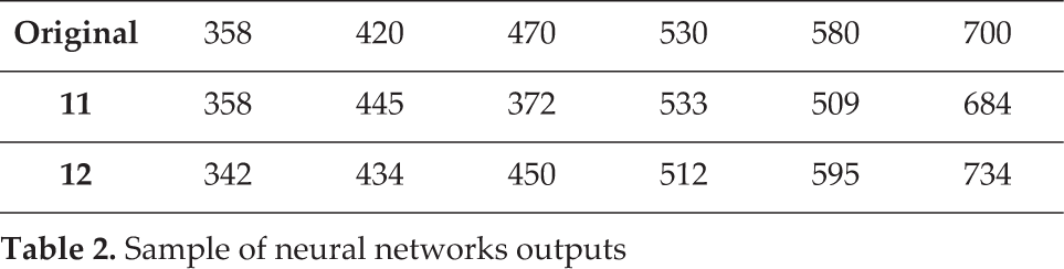
As can be seen from the table 2, the differences between the outputs of individual models of the ANN are not very noticeable, but in some cases the proposed order quantity is disadvantageous for the company. In the third and fifth case, the ordered quantity proposed by the neural network with 11 hidden neurons would be insufficient for the company; it would probably not be able to meet demand, which could lead to a reduction in income and the loss of some customers.

As an ordering system the fixed-time period system is proposed as the most effective ordering structure according to Sanders [30]. The interval between the moments for detecting inventory and setting the order should be determined. For the company under study it is set to three months, in other words, the company will order four times a year as it has done previously.

Table 3 shows the cost per order and storage costs from 2011 to 2014 in financial units (FU). The table contains both the company's actual cost for the goods (reality), and the cost it would incur if it used the proposed ANN model with optimal architecture for decision making (proposal).

Table 3.

Costs related to real and proposed quantity

Year		Transport Costs [FU]	Holding Costs [FU]	Total [FU]	Difference [FU]
2011	Reality	180 679	4 609	185 288
	Proposal	142 125	4 190	146 315	−38 973
2012	Reality	302 302	3 549	305 851
	Proposal	266 935	5 001	271 936	−33 915
2013	Reality	290 861	5 240	296 100
	Proposal	305 810	6 265	312 075	15 975
2014	Reality	563 052	12 840	575 892
	Proposal	382 710	6 776	389 486	−186 406

The table shows that in almost all years there have been marked cost savings for acquiring and holding goods. This is achieved by optimizing the goods ordered in accordance with the expected demand, leading to optimizing the volume of goods held in stock and consequently the storage cost. The cost savings would have only not occurred in 2013. In that year the volume of the company's goods in stock declined too much, often far below the level of safety stock. The company's inability to meet orders is a more dangerous situation than the high cost of goods, and the proposed volume of purchase is still more convenient. In 2014, the company tried to avoid shortages of goods in stock and ordered in larger volumes, which resulted in very high costs both of ordering and storage. Here, the difference between the proposal and the reality is the greatest.

For the ordering cycle, the fixed-time period system is considered. Inventory is monitored in a three-month interval and orders are made according to the actual state of the inventory. Figure 2 shows a comparison of the inventory level based on real values using the proposed model. The diagram clearly shows a more even distribution of the inventory level for values indicated in the model, primarily for 2014. Likewise, the diagram shows that in reality the inventory dropped below the value of 100 units many times, which could mean the company is not able to satisfy its orders.

Figure 2.

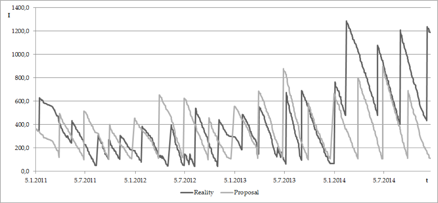
Comparison of inventory level in reality and according to proposal

A comparison of the proposed model and other known methods could be a part of another research project. For now, we can say that the proposed model appears to be more effective than the basic EOQ model. The EOQ model does not work with variable demand within one year.

5. Conclusion

The article examines the possibilities of applying ANN in a company's ordering system. Within the research, the author has developed nine ANN models with different architectures to optimize the order size as a function of the current demand, demand in the next three months, three-month delay demand, current inventory status, purchase cost and procurement costs. The author has used real data of a fasteners wholesaler.

The optimum ANN architecture network found is 6-12-1, i.e., six inputs, 12 neurons in a hidden layer and one output. The performance of the neural network model was evaluated by the coefficient of determination (R²) and the mean squared error.

The ANN model developed can be used to optimize a company's order cycle. Based on the predicted demand and the model designed, it is possible to set up the optimum volume of goods to order and thus improve the inventory management policy in a company for cost of purchasing and storage.

Footnotes

6. Acknowledgements

This paper was supported by grant FP-S-15-2787 ‘Effective Use of ICT and Quantitative Methods for Business Processes Optimization’ from the Internal Grant Agency at Brno University of Technology

References

Nenes

Panagiotidou

Tagaras

. Inventory management of multiple items with irregular demand: A case study. European Journal of Operational Research. 2010;205(2):313–324. DOI: 10.1016/j.ejor.2009.12.

Harris

F. W.

How Many Parts to Make at Once. Factory, The Magazine of Management. 1913;10(2): 135–152.

Novotná

. The impact of the inflation and unemployment values from the previous period on the Phillips curve. In The 7th International Scientific Conference Business and Management 2012; Vilnius Gediminas Technical University Press; 2012. p. 147–158.

Novotná

. Feedback influence on the behavior of the financial System. Economic Computation and Economic Cybernetics Studies and Research. 2014;2014(1):217–231.

Novotná

. Numerical solution of the inventory balance delay differential equation. International Journal of Engineering Business Management. 2015;7DOI: 10.5772/60113

Costantino

Di Gravio

Shaban

Tronci

. Exploring the bullwhip effect and inventory stability in a seasonal supply chain. International Journal of Engineering Business Management. 2013;5:1–12. DOI: 10.5772/56833

Kaur

Sharma

. Inventory model: Deteriorating items with price and time dependent demand rate. International journal of Modern Engineering Research. 2012;2(5):3650–3652.

Ouyang

L. Y.

K. S.

Cheng

M. C.

An inventory model for deteriorating items with exponential declining demand and partial backlogging. Yugo-slav Journal of Operations Research. 2013;15(2): 2334–6043.

Mahata

G. C.

An EPQ-based inventory model for exponentially deteriorating items under retailer partial trade credit policy in supply chain. Expert Systems with Applications. 2012;39(3):3537–3550.

10.

Yadav

A. S.

Gupta

Garg

Swami

. A soft computing optimization based two ware-house inventory model for deteriorating items with shortages using genetic algorithms. International Journal of Computer Applications. 2015;126(13): 7–16.

11.

Al-Khateeb

F. B.

Teng

J. T.

Cárdenas-Barrón

L. E.

Inventory models for deteriorating items with maximum lifetime under downstream partial trade credits to credit-risk customers by discounted cash-flow analysis. International Journal of Production Economics. 2016;171(1): 105–115. DOI: 10.1016/j.ijpe.2015.10.020

12.

Bhunia

A. K.

Shaikh

A. A.

Sahoo

. A two-warehouse inventory model for deteriorating item under permissible delay in payment via particle swarm optimisation. Int. J. Logistics Systems and Management. Forthcoming.

13.

Sana

S. S.

A production-inventory model of imperfect quality products in a three-layer supply chain. Decision Support Systems. 2011;50(2): 539–547.

14.

Sarkar

. An inventory model with reliability in an imperfect production process. Applied Mathematics and Computation. 2012;218(9):4881–4891.

15.

Sarkar

. An improved inventory model with partial backlogging, time varying deterioration and stock-dependent demand. Economic Modelling. 2013;30:924–932.

16.

Ioana

Mirea

Bălescu

. Economic processes study through fuzzy logic. Journal of Economic Computation and Economic Cybernetics Studies and Research. 2012;44(2):129–137.

17.

Zhang

. A Monte Carlo Analysis for stochastic distance function frontier. Inzinerine Ekonomika-Engineering Economics. 2012;23(3):250–255.

18.

Gaafar

Choueiki

M. H.

A neural network model for solving the lot-sizing problem. Omega. 2000;28(2):175–184.

19.

Megala

Jawahar

. Genetic algorithm and Hopfield neural network for a dynamic lot sizing problem. The International Journal of Advanced Manufacturing Technology. 2006;27(11–12): 1178–1191.

20.

Šenyiğit

Düğenci

Aydin

Zeydan

. Heuristic-based neural networks for stochastic dynamic lot sizing problem. Applied Soft Computing. 2013;13(3):1332–1339.

21.

Baciarello

D'Avino

Onori

Schiraldi

. Lot sizing heuristics performance. International Journal of Engineering Business Management. 2013;5:1–10. DOI: 10.5772/56004

22.

Baki

Chaouch

Abdul-Kader

Baki

Chaouch

Abdul-Kader

. A heuristic solution procedure for the dynamic lot sizing problem with remanufacturing and product recovery. 2014;43:225–236. DOI: 10.1016/j.cor.2013.10.001

23.

Schulz

. A new silver-meal based heuristic for the single-item dynamic lot sizing problem with returns and remanufacturing. International Journal of Production Research. 2011;49(9):2519–2533. DOI: 10.1080/00207543.2010.532916

24.

Beck

F.G.

Grosse

E.H.

Teßmann

. An extension for dynamic lot-sizing heuristics. Production & Manufacturing Research. 2015;3(1):20–35. DOI: 10.1080/21693277.2014.985390

25.

Kang

H.Y.

Lee

A.H.

A stochastic lot-sizing model with multi-supplier and quantity discounts. International Journal of Production Research. 2013;51(1):245–263. DOI: 10.1080/00207543.2012.674649

26.

Hamzaçebi

. Improving artificial neural networks' performance in seasonal time series forecasting. Information Sciences. 2008;178(23): 4550–4559. DOI: 10.1016/j.ins.2008.07.024

27.

Hachicha

. A simulation metamodelling based neural networks for lot-sizing problem in MTO sector. Journal of Simulation Modelling. 2011;10(4): 191–203. DOI: 10.2507/IJSIMM10(4)3.188

28.

Paul

S. K.

Azaeem

. An artificial neural network model for optimization of finished goods inventory. International Journal of Industrial Engineering Computations. 2011;2(2):431–438. DOI: 10.5267/j.ijiec.2011.01.005

29.

. An inventory controlled supply chain model based on improved BP neural network. International Journal of Industrial Engineering Computations. 2013;2013:1–7. DOI: 10.1155/2013/537675

30.

Sanders

. Operations Management Defined [Internet]. 23 January 2014. Available from: http://www.ftpress.com/articles/article.aspx?p=2167438&seqNum=7. Accessed on 04 Mar 2016.

An Artificial Neural Network Model for a Wholesale Company's Order-Cycle Management

Abstract

Keywords

1. Introduction

2. Literature Review

3. ANN Model

4. Results and Discussion

5. Conclusion

Footnotes

6. Acknowledgements

References