
Abstract
This paper presents a dynamic model for a self-balancing vehicle using the Euler-Lagrange approach. The design and deployment of an artificial neuronal network (ANN) in a closed-loop control is described. The ANN is characterized by integration of the extended delta-bar-delta algorithm (DBD), which accelerates the adjustment of synaptic weights. The results of the control strategy in the dynamic model of the robot are also presented.
Keywords
1. Introduction
The development of heuristic control algorithms for intelligent robots is common practice today. Since these control strategies do not require the dynamic model of any given system, previous knowledge of such a system is sufficient for implementing control algorithms. The adaptive properties of ANNs give rise to the possibility for achieving control strategies for systems with unknown and random disturbances. The self-organization of ANNs, i.e., the ability to modify the entire network to fulfil a specific task, enables the algorithm's capability of adequately reacting to unexpected circumstances [10].
Similarities between wheeled inverted pendulum (WIP) systems and human posture has become the primary reason for the study of these systems in recent years [9]. In 2001, the Segway PT© was commercially released as a personal transport vehicle. The Segway uses the WIP principle and is capable of reaching a speed of 20.1 km/h [5]. Most control strategies proposed for WIP systems use model-free control strategies, in which the purpose of a dynamic model is only to evaluate the behaviour of the control algorithm and therefore, the dynamic model is not part of the control strategy [15, 13].
Dynamic models as part of the controller's algorithm and the combination of theoretical models with a heuristic approach have been studied in the past. A control strategy based on two decoupled state-space controls that are obtained from a mathematical model which, in turn, is obtained from the physical characteristics of the robotic platform, has been reported [8], where one control strategy is used for pitch and the other for yaw. Additionally, a Tagaki-Sugeno fuzzy control was designed and implemented [1] for a WIP system. This strategy combines heuristic knowledge and information from the dynamic model in order to maintain a robot in the vertical position. Furthermore, this approach allows for motion of the WIP over ascending slopes. Other approaches have also considered this issue [2, 3].
A controller consisting of two ANNs with a radial basis function in the control loop has been presented [6], one for pitch and the other for yaw. This work demonstrates the adequate performance of the controller for low velocities. A neural adaptive output feedback control has been reported [6]. This framework incorporates a linear dynamic compensator in order to increase the vertical stability of a WIP robot, while allowing for the tracing of paths.
Several techniques have been proposed for deriving the dynamic equations of motion in WIP systems, including Newton equations [8], Lagrangian equations [4, 12], non-holonomic constraints [13, 7] and the addition of these constraints alongside Boltzman-Hamel equations [14]. In the present work, a dynamic model is obtained using the Euler-Lagrange equations.
2. Dynamic Model
In order to obtain the dynamic model of the proposed system it was assumed that:
The robot moves over a flat surface.
The wheels are perpendicular to the ground.
The robot's body behaves as a rigid body.
According to the free-body diagrams depicted in Fig. 1 and in Fig. 2, the self-balancing robot consists of three elements: the two wheels and the robot's body. The chosen parameters for the dynamic model are summarized in Table 1.
System parameters


Side view of the free-body diagram

Top view of the free-body diagram
The proposed modelling method, an Euler-Lagrange approach, defines a set of differential equations describing the time evolution of a mechanical system under holonomic constraints [9]. This methodology requires the definition of the generalized coordinates vector, the calculation of the kinetic energy of the system, definition of the potential energy, computation of the Lagrangian and finally, establishment of the differential equations.
2.1. Generalized coordinates vector
Information-carrying variables of the degrees-of-freedom define the generalized coordinates vector. In our study, the coordinates vector is defined as:

where θ represents the angle with respect to the vertical component, φ is the rotational angle of the robot with respect to the reference plane and d is the displacement of the robot.
2.2. Kinetic energy
It is known that the body masses in the robot are subject to rotational inertia, which contributes to the acceleration of the body masses. Hence, the kinetic energy can be established as:
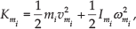
where mi represents the body masses in the robot, vi represents the velocity of each corresponding mass,
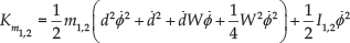
The overall kinetic energy of the system becomes the sumatory of the kinetic energy in each body mass. Therefore

where
and

2.3. Potential energy
Since the energy of the proposed configuration depends on the vertical position and mass of the robot, the force applied by the gravitational potential energy can be expressed as

where U is the potential energy, mi is the corresponding mass, g is the acceleration of gravity and y is the distance from the origin of the reference frame to the centre of mass. Similar to kinetic energy, the total potential energy is the sumatory of the potential energy contained in each body mass. Hence, for our proposed configuration:
where

and

2.4. Lagrangian
The Lagrangian is defined as the difference between the total kinetic energy (3) and the total potential energy (7). Hence:

Consequently,

2.5. Euler-Lagrange equation
Once the Lagrangian has been defined, the Euler-Lagrange equation for each element in the generalized coordinates vector is required. Therefore:

where
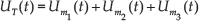
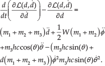
According to (1), the WIP robot has three parameters that lead to three differential equations. These equations are obtained by replacing q and

Then,

Also,
Arranging the generalized acceleration and velocity vectors, equations (12), (13) and (14) can be expressed as follows:

where
For the WIP system, matrices in (15) are established as follows:

where,
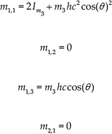
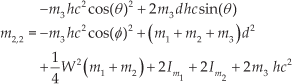


then,
where,


and

where,


2.6. Dynamic model verification
A number of properties must be fulfilled in order to validate the proposed model [9, 11]. This section describes these properties.
The inertia matrix


Value of the determinant of
The inverse of the inertia matrix

Value of the determinant of
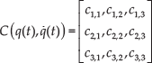
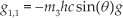
Dynamic equations contain terms from the generalized coordinates vector

where,
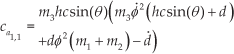


Every element in (17) is multiplied by a component in the generalized velocities vector; therefore,
Regardless of how

where
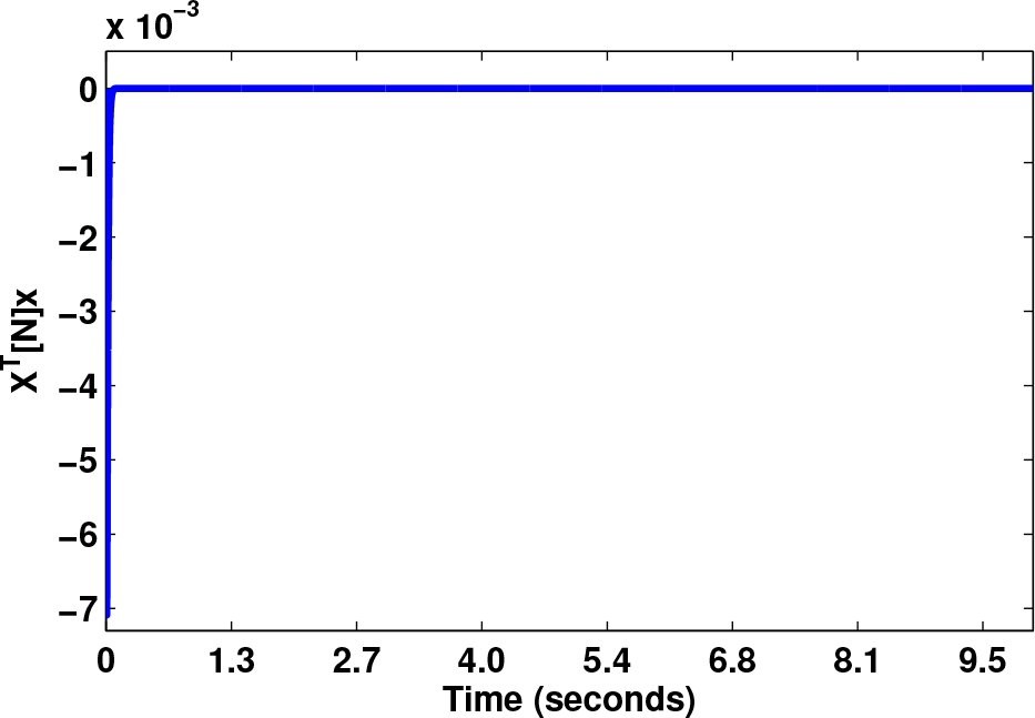
Behaviour along a defined path at a 10 second duration
It can be observed that the boundary conditions force a non-zero value in the beginning of the simulation. Immediately after this condition passes, a zero value can be observed. The gravitational forces vector

Therefore,

Once the model has been verified using the aforementioned properties, it can be stated that the mathematical approximation obtained by the Euler-Lagrange approach is appropriate for the control strategy proposed in the following section.
3. Control Design
A multi-variable recurrent neural network, in which recurrence is set in the hidden layer, is proposed as a control strategy for the WIP system. Fig. 6 shows the general outline of the control strategy. Parameters yd and yr represent the desired and actual angular position of the WIP system, respectively. These two parameters are one-dimensional vectors. In Fig. 6, the error
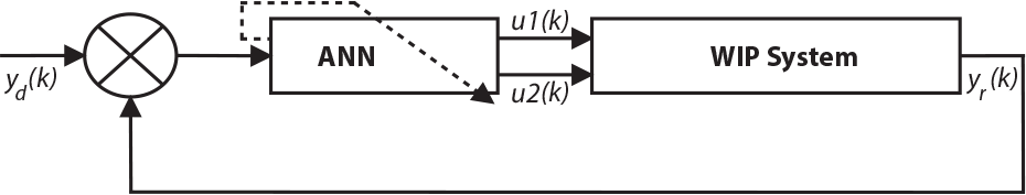
Control strategy outline with the ANN
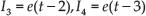
The ANN consists of four inputs (the most recent

General scheme of the ANN
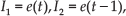
Inputs Ii are defined as:
At the input of each neuron, a weighted sum is performed by multiplying the input variable by its synaptic weight. This weighted sum, denoted by

where

Since no limit in the output values is required, a linear activation function in the output layer is specified as:

Backpropagation learning requires an error function that depends on the synaptic weights; concurrently, this function must be capable of evaluating the performance of the network. An iterative minimization of such a function will result in a general method for optimizing the synaptic weights. The proposed function is:

The chosen optimization method uses gradient descent, as this takes the first derivative of the error function

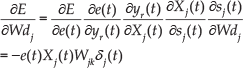
The update of the synaptic weights is performed by using the following:

equation (30) is substituted in

where η represents the learning factor and

The weight-updating function in the hidden layer is:

The recurrent synaptic weights
By substituting (35) in (31) the update of

Gradient descent for

Finally, the update of

The response of θ, the variable to be controlled, after applying the ANN algorithm is depicted in Fig. 8. The initial conditions are:
Simulation response of
The main objective of a control loop for a WIP system is to maintain a vertical position (
After carrying out a strict analysis of the performance of the ANN, compensation of the error produced by θ is observed. However, when the error sign changes from positive to negative, the compensation of the control loop is too slow, because the learning factor is too small. In other words, when a sudden change in θ occurs, the network fails to adapt and hence, is unable to control the system.
3.1. Extended delta-bar-delta algorithm
The delta-bar-delta algorithm is a heuristic approach that can be used to improve the convergence speed of the weights in ANNs. The weights are updated by:

where

where θ is the convex weighting factor. The learning coefficient change is given as:

where ν is the constant learning coefficient increment factor and θ is the constant learning coefficient decrement factor. However, knowing how to choose the heuristic parameters is not a straightforward task. Therefore, implementing this algorithm online is not feasible [16].
The extended delta-bar-delta (EDBD) algorithm is an extension of the delta-bar-delta (DBD) algorithm. In the EDBD, the changes in weights are calculated from:

and the weights are then found as:

In Eq. 41,

where να is the constant momentum coefficient scale factor,
An extended delta-bar-delta algorithm is then used to solve the adaptation issue of the ANN. The algorithm adds a learning factor for each synaptic weight, allowing for an adaptation when the control variable presents a sign change. The simple DBD algorithm provides a suitable speed-up. However, this presents some disadvantages. For instance, when using momentum alongside DBD, the algorithm may diverge dramatically. When k is small, the learning rate may increase. Therefore, when the algorithm decreases exponentially, it may not be able to handle sudden sign changes. The EDBD algorithm is implemented by adding (31) and the momentum terms [17]. The proposed equation is then:

where i is the neuron number in the previous layer and j is the neuron number in the consecutive layer. Hence,


Parameters
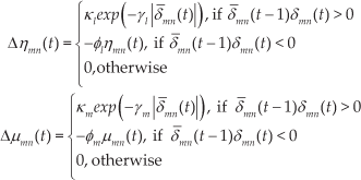
κl, φl, γl, κm, φm and γm are parameters defined by the control designer.
4. Controller Simulation with a Dynamic Model
A set of initial values for the system parameters were defined; following on, heuristic optimization was performed. Table 2 summarizes the parameters.
Parameters of the EDBD algorithm for the ANN

Synaptic weights
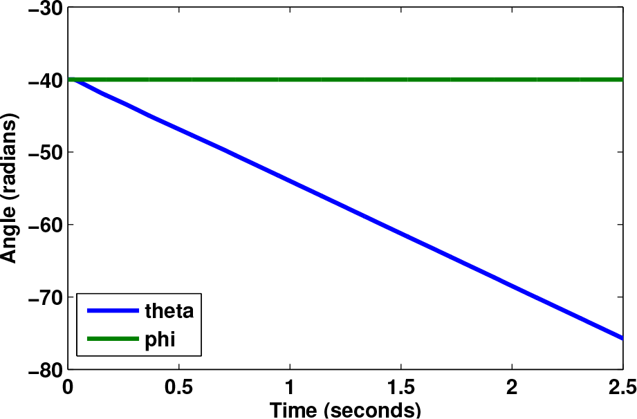
The simulation results shown in Fig. 9 prove that the controller is capable of maintaining the value of θ between
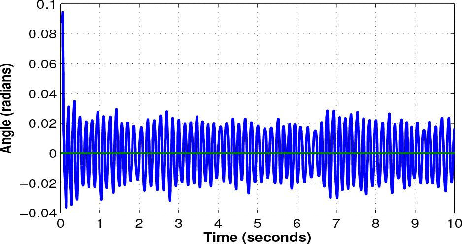
Simulation response of the ANN controller for θ and φ

System displacement response of the ANN controller
The control output signal is the same for both output neurons because there is only one variable to control and as a consequence, only one error parameter
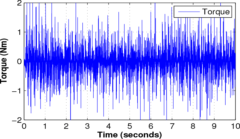
Torque applied to the system
Fig. 12 shows the performance of the ANN during the first second; the average torque value is within

Applied torque to the system, first second
Several simulation runs were carried out, changing the initial value of θ from
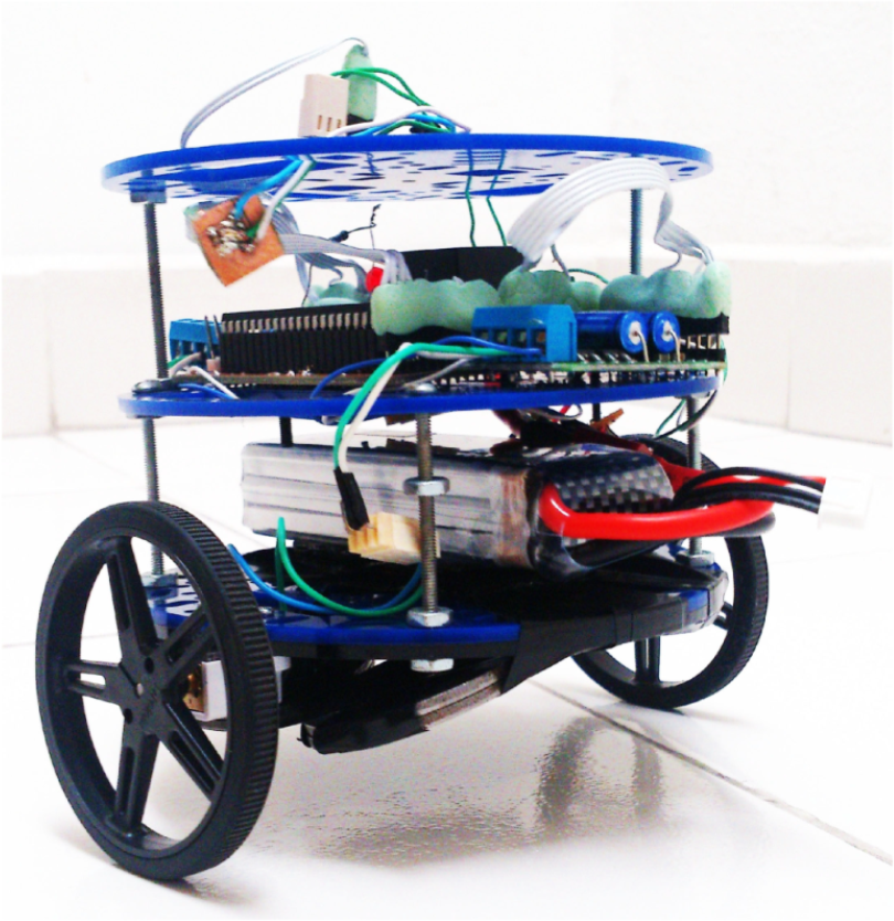
Photograph of the self-balancing vehicle
5. Conclusions
A control strategy that does not require the dynamic model of a WIP system was proposed. The reported control strategy focuses on a small variation range for the variable to be controlled. This control strategy can be combined with other strategies to work within a wider range. Since conventional PID-based controllers may experience a small but noticeable oscillation around the desired set point, it was proven that external disturbances can be successfully compensated for by using a dynamic learning factor for the synaptic weights. This dynamic factor significantly improves the adaptation process at each iteration of the ANN controller. This improvement was possible through the addition of the extended EDBD algorithm.
Footnotes
6. Acknowledgements
The authors acknowledge the financial support provided by the Mexican National Council for Scientific and Technological Development and the Department of Applied Research at the Centre for Engineering and Industrial Development. Additionally, this work was partially funded by the CONACYT grant 163660.