Sage Journals: Discover world-class research

Abstract

In this study, a series of new concepts and improved genetic operators of a genetic algorithm (GA) was proposed and applied to solve mobile robot (MR) path planning problems in dynamic environments. The proposed method has two superiorities: fast convergence towards the global optimum and the feasibility of all solutions in the population. Path planning aims to provide an optimal path from a starting location to a target location, preventing collision or so-called obstacle avoidance. Although GAs have been widely used in optimization problems and can obtain good results, conventional GAs have some weaknesses in an obstacle environment, such as infeasible paths. The main ideas in this paper are visible space, matrix coding and new mutation operators. In order to demonstrate the superiority of this method, three different obstacle environments have been used and an experiment is conducted. This algorithm is effective in both static and dynamic environments.

Keywords

Visible Space Genetic Algorithm Matrix Encoding Mutation Chromosome Modification Path Planning

1. Introduction

Path planning is a crucial issue in artificial intelligence and MR domains. The issue concerns the search for feasible paths for MRs to move from a start location to a target location in an environment with obstacles [1]. The path planning environment can be either static or dynamic [2]. In the static environment, everything is static except the MR. Before a robot moves towards the target, the nearest feasible path must be obtained. However, one or more obstacles would be intersected, while the computation processes are complicated. Researchers have been searching alternative and more efficient ways to solve the path planning problems [3].

Many techniques and algorithms have been applied to solve path planning problems, such as grid-based A* algorithms [4 –6], road maps (Voronoi diagrams and visibility graphs) [7,27, 28], D* algorithms [8, 29 –31], fuzzy logic [9], genetic algorithms [2], particle swarm algorithms [10], PBIL algorithms [11], ant colony algorithms [12], simulated annealing [13], potential field methods [14, 15] and so on. Each has its merits and drawbacks in different environments. For example, an A* algorithm can acquire a solution faster than a GA in relation to small-scale maps.

GAs were first proposed by Holland [16], informed by the theory of evolution [17]. In other words, they are inspired by biological evolution and have proved to be robust and powerful adaptive search techniques [18]. Indeed, GAs have been successfully applied to optimization problems in many domains.

A dynamic robot path planning schema for unknown environments is studied in [19]. In [20], GAs are used to generate the optimal path by exploiting the advantage of its strong optimization ability, leading to the proposal of a tailored genetic algorithm for optimal path planning. GAs have attracted considerable interest due to their usefulness in solving complex robot path planning problems [11].

However, GAs also have some shortcomings, for example, slow convergence rates, local optima and ignoring cooperation between populations [21].

Based on the advantage of other optimization algorithms, many researchers have studied hybrid genetic algorithms. A hybrid of an ant colony algorithm and a GA can reduce the risk of falling into a local minimum and minimizing the execution time. [22] studied the use of a hybrid multi-neuron heuristic search and genetic algorithm. Other researchers have concentrated on modifying operators belonging to GAs. Adem Tuncer in [2] improved a new mutation operator and applied it to the path planning problem for an MR; good results were obtained.

In light of the previous studies, some new methods are proposed for solving path planning problems for an MR in this paper. It involves an improved GA, as well a new population generation strategy, a novel environment representing and encoding method, and novel mutation operators. The proposed improved genetic algorithm (IGA) allows the MR to navigate in a dynamic environment without being trapped. Comparisons with A*, D* and two IGAs are summarized in Table 1.

This article is organized as follows. In section 2, some preconditions are listed and the concept of visible space is described. In section 3, the proposed IGA is described in detail. In section 4, experiments are performed in order to make a comparison between the proposed method and A*, D* and two IGAs. A conclusion of this paper is given in section 5.

Table 1.

Comparison between the proposed IGA and A*, D* and the other IGAs

	A*	D*	IGA in reference [2]	IGA in reference [26]	This paper
Global planning	✓	✓	✓	✓	✓
Small time consumption in large scale		✓			✓
Power of convergence			✓		✓
Highly scalable		✓			✓
Adaptability in dynamic environment		✓	✓	✓	✓

2. Concept of Visible Space

Since GAs have been frequently used, this paper will not describe the basic GA as referenced in [2, 23, 24,26]. Rather, this paper focuses on visible space, new mutation operators and the modification method of infeasible genes.

2.1. Assumptions

To simplify the path planning problem, it is necessary to make some assumptions. They are as follows:

At least one path along which a robot can move from a start location to a target location is available.

The obstacle space is known.

All obstacles are made up of unit grids, whether regular or irregular, as shown in Figures 2 and 3.

This improved algorithm is represented in a two-dimensional (2D) space.

The path point is always the centre of a grid.

In order to simplify calculation, amplification is carried out in relation to the obstacles.

According to the upper assumption f, the robot can be considered as a particle without considering its dimensions.

2.2. Problem space representation

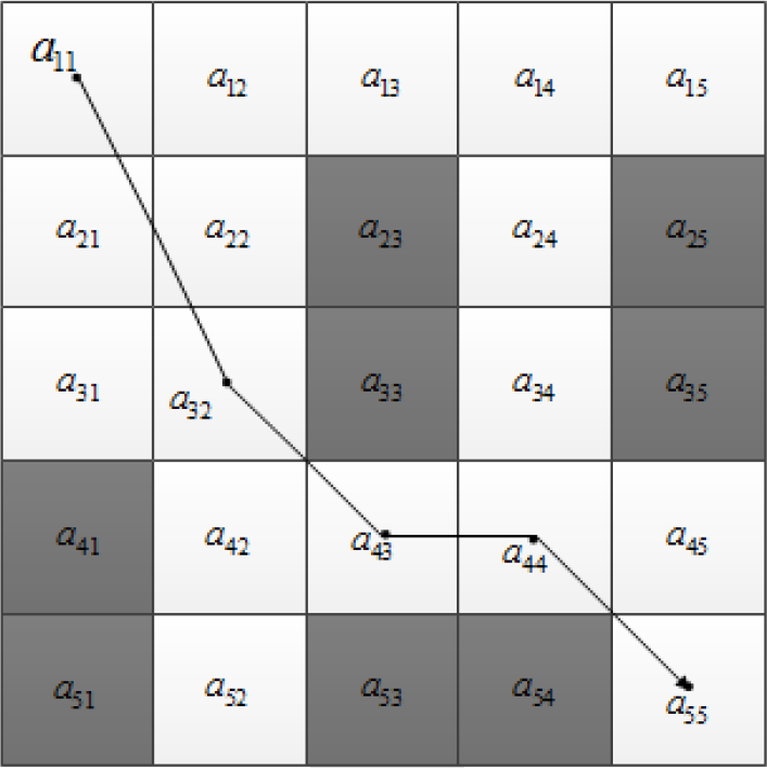
Many path planning methods for MRs use a grid-based graph to represent the obstacle space, as shown in Figure 1. This paper takes the same approach, but with a different encoding method. In Figure 1, the darker colours represent obstacles, while the lighter colours represent obstacle-free spaces.

Some methods in the literature use orderly numbered encoding to represent the relative position of grids [2]. When applying the methods in the literature, a decoding operation is required. A matrix encoding method is applied in this paper; therefore, there is no need to decode. In this method, the position of a grid is reliant upon its row index and column index. For example, a grid $a_{i j}$ in an obstacle space stands for the position in row i and column j.

In this matrix encoding method, the problem space is indicated in Figure 1. According to an arbitrary grid within an obstacle problem, its position can be obtained from its subscript, as well as the positions of eight neighbourhood grids. In this paper, visible space can be obtained according to the relative positions of grids.

Figure 1.

An example using the matrix encoding method to represent the obstacle environment

2.3. Concept of visible space

As light travels in straight lines, no one can see the object behind the obstacles. Based on the Markov process, the position of a path waypoint only depends on its previous waypoint. An environment space $S_{m \times n}$ includes the obstacles $Ω = {o_{1}, o_{2}, \dots, o_{p}}$ , while the obstacle free spaces are $B = {b_{1}, b_{2}, \dots, b_{q}}$ and an equation is $p + q = m \times n$ . If an MR stands at $a_{i j} \in B, (1 \leq i \leq m, 1 \leq j \leq n)$ , $V_{i j}$ is a set of the obstacle-free grids that can be derived from $a_{i j}$ , while $V_{i j}$ is the visible space of grid $a_{i j}$ .

If an MR tries to obtain a path from the starting point to the target point, the path waypoint from current visible space $V_{i j}$ should be selected. After a number of iterations, a feasible path can be obtained.

This concept seems similar to the visibility map method in [10], even though they are different concepts. The visibility map method can obtain globally optimal solutions; however, when the environment has changed, much time is required for re-calculation. Meanwhile, the method in this study is only concerned with obstacles in front of the MR, which means the complexity can be reduced.

2.4. Method to obtain visible space

In an obstacle environment, obstacles can be all kinds of shape, but only a small number of vertices play a decisive role in the line of sight. In Figure 2, there are three types of vertices in an obstacle, but only vertices marked with red circle 1 have an effect on visible space calculation.

To obtain visible space, three steps are required: first, the obstacles that impact on the line of sight most obviously need to be obtained (these obstacles are called the “outer envelope”); second, vertices that have an effect on calculation need to be obtained (the action is a further simplification process); and third, obstacle-free grids as visible space can be obtained.

2.4.1. Method to obtain the “outer envelope”

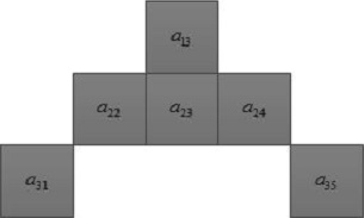
Before the optimization operations, the obstacle environment and the shape of each obstacle must be known. Owing to the matrix representation, the shapes and positions of obstacles can be obtained quickly. In this paper, a new concept of the “outer envelope” is proposed, which is important to visible space calculation; see Figure 2.

The “outer envelope” will be explained by the example in Figure 2. There exists an obstacle consisting of nine grids, $O = {a_{22}, a_{23}, a_{24}, a_{32}, a_{33}, a_{34}, a_{42}, a_{43}, a_{44}}$ , and a current path waypoint S ( $a_{51}$ ). When $a_{51}$ is connected to the upper left vertex of grid $a_{22}$ as line segment 1 and $a_{51}$ is connected to the lower right vertex of $a_{44}$ as line segment 2, the grids between these two line segments and at the back of the obstacles cannot simultaneously be reached via the current path point directly. Other grids are visible, which can be reached. In Figure 2, line segments 3 and 4 obviously have no effect on visible space calculation. This is what we find in the “outer envelope” of obstacles. A very important note is that, if the current position has changed, the visible space may change too, even though the outer envelope does not. The steps to obtain an “outer envelope” are shown in Table 2.

Table 2.

Steps to obtain an “outer envelope”

Step	Operation
1	The row indices are sorted in ascending order as a set of $X_{1}$ .
2	If the value of $a_{i j}$ in $X_{t} (t = 1, 2)$ changes from 0 to 1 or from 1 to 0, this point is a transition point and can be reserved in $X_{i}$ . (The value of obstacle is 1 and the value of other grids is 0).
3	The column indices are sorted in an ascending order as a set of $X_{2}$ , and repeat the step2.
4	Taking an intersection $X = \cap_{t = 1}^{2} X_{t}$ , and X is the “outer envelope”.

This is a general method to obtain an “outer envelope” of obstacles. No matter how complex or large it is, obstacles can be simplified by this method. “Outer envelopes” are always on the outside of obstacles, which means that this method can obtain them quickly.

Figure 2.

An example of an “outer envelope”

Here is a simple example to illustrate how to get an “outer envelope” for an obstacle: the obstacle is in Figure 2 and the specific steps are in Table 3.

Table 3.

Instance of steps to obtain an “outer envelope” as shown in Figure 2

Step	Operation
1	The row indices are sorted in ascending order X₁={a₂₂a₂₃a₂₄a₃₂a₃₃a₃₄a₄₂a₄₃a₄₄} .
2	The transitional grids are reserved X₁'={a₂₂a₂₄a₃₂a₃₄a₄₂a₄₄} .
3	The column indices are sorted in ascending order X₂={a₂₂a₃₂a₄₂a₂₃a₃₃a₄₃a₂₄a₃₄a₄₄} .
4	The transitional grids are reserved X₂'={a₂₂a₄₂a₂₃a₄₃a₂₄a₄₄} .
5	Taking an intersection of X₁' and X₂', the “outer envelope” a₂₂a₄₂a₂₄a₄₄ is obtained.
6	The result of step 5 is sorted in row index ascending order, and the final result is a₂₂a₂₄a₄₂a₄₄ .

This method is also suitable for the concave polygon, as shown in Figure 3, in which the “outer envelope” is $X = {a_{13} a_{22} a_{24} a_{31} a_{35}}$ .

2.4.2. Method to obtain effective vertices

The amount calculated is still large after “outer envelopes” are obtained. The next step is to obtain effective vertices of the grids. If $a_{i j}$ is a grid in an obstacle environment, there are five key points that need to be mentioned as follows:

Lower left vertex: $(i - 1, j - 1)$ .

Lower right vertex: $(i, j - 1)$ .

Upper left vertex: $(i - 1, j)$ .

Upper right vertex: $(i, j)$ .

Centre: $(i-1/2,j-1/2)$

This method can convert the subscript of a grid in a problem space to a 2D coordinate system in the xy-plane. At this moment, the four vertices of a grid can be obtained, but not all vertices have an effect on the visible space calculation. Therefore, further simplifying is necessary, such as grid $a_{22}$ , which has four vertices in Figure 2, but only vertex (1, 2) is useful.

Figure 3.

An example of a concave polygon

According to the relative positions of eight neighbourhood grids, the following equations can be obtained. $a_{s k}$ is one of the eight neighbourhood grids of $a_{i j}$ .

| i - s | = 0 & & (j - k) = 1

(1)

| i - s | = 0 & & (j - k) = - 1

(2)

(i - s) = 1 & & | j - k | = 0

(3)

(i - s) = - 1 & & | j - k | = 0

(4)

(i - s) = 1 & & (j - k) = 1

(5)

(i - s) = 1 & & (j - k) = - 1

(6)

(i - s) = - 1 & & (j - k) = 1

(7)

(i - s) = - 1 & & (j - k) = - 1

(8)

n_{s k} (e) = N, e = 1, 2, 3, \dots, 8

(9)

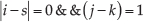
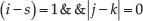
Eqs. (1) and (2) indicate that grids $a_{i j}$ and $a_{s k}$ are on the same row. Eqs. (3) and (4) indicate that the two grids are in the same column. Eqs. (5), (6), (7) and (8) indicate that the two grids are on diagonal lines. These eight equations can demonstrate the relative position of the grids.

In Eq. (9), N equals 0/1. If $n_{s k} (e) = N = 0$ , this indicates that $a_{i j}$ and $a_{s k}$ are not satisfying Eq. (e). Meanwhile, if $n_{s k} (e) = N = 1$ , this indicates that $a_{i j}$ and $a_{s k}$ are satisfying Eq. (e). The actual conditions are in Table 4.

Table 4.

Vertices and obstacle relations

Conditions	Effective vertices	Position description
$n_{s k} (1) = 1$	$(i, j - 1)$ , $(i, j)$
$n_{s k} (2) = 1$	$(i - 1, j - 1)$ , $(i - 1, j)$
$n_{s k} (3) = 1$	$(i - 1, j)$ , $(i, j)$
$n_{s k} (4) = 1$	$(i - 1, j - 1)$ , $(i, j - 1)$
$n_{s k} (5) = 1$	$(i, j - 1)$ , $(i - 1, j)$ , $(i, j)$
$n_{s k} (6) = 1$	$(i - 1, j - 1)$ , $(i - 1, j)$ , $(i, j)$
$n_{s k} (7) = 1$	$(i - 1, j - 1)$ , $(i, j - 1)$ , $(i, j)$
$n_{s k} (8) = 1$	$(i - 1, j - 1)$ , $(i, j - 1)$ , $(i - 1, j)$

Meanwhile, the effective vertices can be obtained by using the following equation:

C_{i j} = \cap_{e = 1}^{8} (n_{s k} (e) = 1)

(10)

2.4.3. Method to obtain the visible space of the current position

According to the above methods, every effective vertex in relation to obstacles can be obtained. When the centre of current point $a_{i j}$ is connected with these effective vertices in $C_{i j}$ , a set of line segments $L_{i j}$ can be obtained. The angle between these lines can be marked as $(A^{o}_{θ \min}, A^{o}_{θ \max})$ , where o represents the $o - t h$ obstacle, $A^{o}_{θ \min}$ is the minimum angle between a line segment in $L_{i j}$ and the coordinate axis, $A^{o}_{θ \max}$ is the maximum angle between a line segment in $L_{i j}$ and the coordinate axis, and $A^{o}_{θ \max} - A^{o}_{θ \min}$ is the maximum angle between these line segments.

Grids that are between the maximum angle $A^{o}_{θ \max} - A^{o}_{θ \min}$ but also behind corresponding obstacles cannot be reached. The other obstacle-free spaces can be reached.

As Figure 2 illustrates, the visible space of current point $a_{51}$ is:

V_{51} = {a_{11}, a_{21}, a_{31}, a_{41}, a_{52}, a_{53}, a_{54}, a_{55}}

By choosing one point from $V_{51}$ , a new waypoint is obtained.

3. An Improved Genetic Algorithm

3.1. Chromosome encoding

The encoding method is one of the key steps in the design of a GA. The widely used encoding methods include binary encoding, the Gray code, the floating number code and the real number code.

A variant on the character encoding method with a variable length strategy is used in this paper.

Figure 4.

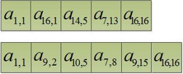
Chromosome encoding strategy

As shown in Figure 4, there are two chromosomes, or paths: $a_{1, 1}$ is the initial position and $a_{16, 16}$ is the target position. The advantage here is that this method does not need to be decoded and contains more information.

3.2. Initialization of population

The population initialization in this paper is based on the concept of visible space. In an obstacle space, robots need to avoid obstacles.

When an MR moves from a starting point, a new waypoint can only be selected from the current visible space. After several iterations, the target point exists in the visible space. A new path is formed by the selected path points; the specific process is shown in Table 5.

In Table 6, a comparison of methods to acquire the initialization population is shown; the simulation scenario is Map 6 in section 4.1. According to the results, the method in this study can obtain an initialization population more quickly than that in [2].

Table 5.

Pseudocode of the initial solution

1. Begin 2. Initializing and setting the environment, population scale N_pop, the maximum iteration of GA N, number of obstacles N_obs, layout of every obstacle L_i, the crossover probability p_c, the mutation probability p_m, the additional mutation probability p_am, the whole population set P. 3. Starting position is PP_c, and target position is PP_t. 4. Calculate visible space of PP_c, record as V_c. 5. Set a counter i = 0. 6. While i < N_pop do. 7. Set a list L_i which is used to store path point. 8. Add PP_c into L_i. 1. Two intermediate-parameters PP_i = PP_c, and V_PPI = V_C. 9. While PP_t ∉ V_PPI do. 10. Select a path point PP_s from V_PPI, and PP_i = PP_s. 11. V_PPI = Calculate visible space of PP_i. 12. End do. 13. Add PP_t into L_i. 14. Add L_i into population P. 15. i = i + 1. 16. End do. 17. Output the path, then begin genetic operation. 18. Set a counter j = 0. 19. While j < N do 20. Calculate chromosome fitness in population. 21. Perform the selection operation, the new population is P_new. 22. Perform crossover operation. 23. If (the crossover point can cause infeasible solution) then 24. Modify the chromosome based on visible space 25. End if 26. Perform mutation operation. 27. Perform additional mutation. 28. If (the additional mutation point can cause infeasible solution) then 29. Modify the chromosome based on visible space 30. End do 31. Output the global optimal solution. 32. MR starts moving. 33. While the MR has not arrived the target position do. 2. If (the environmental change is detected) then. 34. Re-plan the path. 35. End if. 36. End do.

Table 6.

Comparison of the initial solution results information

Function	IGA in reference [2]	IGA in reference [26]	This study
The best fitness	24.01	23.51	23.38
Population size	40	40	40
Number of infeasible solution	0	0	0
Solution Time(s)	3.87	5.87	2.62

3.3. Selection operation

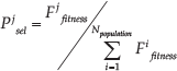
The main principal of the GA is the survival of the fittest, which means chromosomes with the best fitness should survive and be transferred to future generations. The classical roulette selection method is adopted in this paper. If a chromosome has a larger fitness value, a higher likelihood will be selected.

3.4. Fitness function or evaluation function

The fitness function determines how good a chromosome is within a population. Generally speaking, a fitness function is transformed from the objective function. The selection of the fitness function influences the convergence of the algorithm.

The challenge implicit in the path planning problem is to obtain an optimal path, in which the final solution must be the shortest and most feasible.

F_{j} = \min (\sum_{i = 1}^{n} f (i, i + 1)), n = N_{l e n g t h} - 1, j \in [1, N_{p o p u l a t i o n}]

(11)

f (i, i + 1) = \sqrt{{(y_{i + 1} - y_{i})}^{2} + {(x_{i + 1} - x_{i})}^{2}}

(12)

F^{j}_{f i t n e s s} = \frac{1}{F_{j}}

(13)

P^{j}_{s e l} = \frac{F^{j}_{f i t n e s s}}{\sum_{i = 1}^{N_{p o p u l a t i o n}} F^{i}_{f i t n e s s}}

(14)

In Eq. (11), i is the index of the path point in a chromosome. $f (i, i + 1)$ is the length of two path waypoints with index i and $i + 1$ . j is a chromosome in the population. $N_{w a y - p o int}$ is the total number of waypoints in a path. In Eq. (12), ( $x_{i}$ , $y_{i}$ ) is the position of waypoint i, while $x_{i + 1} y_{i + 1}$ is position of the next waypoint. In Eq. (13), a reciprocal value of an objective function is obtained. Eq. (14) is the probability a chromosome to be selected.

3.5. Crossover operation

In the case of infeasible solutions in a population, some researchers have included punitive factors in these infeasible solutions. When the selection operator works, the infeasible solutions have an extremely low probability of being selected. Even if they are selected, their filial generation has a higher probability of being infeasible, which results in a decrease in population diversity.

Although initial solutions in this paper are all feasible, a few infeasible solutions may be obtained after a crossover or mutation operation. Where their parents are all feasible, the infeasible gene only appears at the crossover or mutation point.

Generally speaking, GAs use crossover to exchange genetic material. A single-point crossover operator is applied in this study, with genes of two chromosomes after the crossover point being swapped. The crossover operation is shown in Figure 5.

Figure 5.

Crossover operation

As Figure 5 illustrates, the length of two parents used in a crossover operation can be different.

After the crossover operation, filial generations may contain infeasible genes; the method to solve this situation is given in section 3.8.

3.6. Mutation operator

Mutation, which is one of the most important operators in GAs, is used to maintain diversity in the population and avoid premature convergence.

In conventional GAs, random mutation is the most commonly used operator. However, random mutation can lead to infeasible paths, slowly converging and leading to local optimum.

Two new mutation methods are proposed in this paper, which can ensure converging towards the global optimum.

Figure 6.

Comparison of mutation methods

Table 7 shows the steps of the mutation operation.

Table 7.

Steps of the mutation operation

Step	Operation
1	Selecting one way-point from a chromosome, which is neither a starting point nor a target point, and marked as P_m .
2	The two neighbors of P_m are obtained, marked as P_b and P_t .
3	The line between P_m and P_b is L₁, while the line between P_m and P_t is L₂ .
4	The grids that crossed by L₁ and L₂ are marked as S₁ and S₂ .
5	Two grids are chosen from S₁ and S₂ separately, and connected as a new path way.

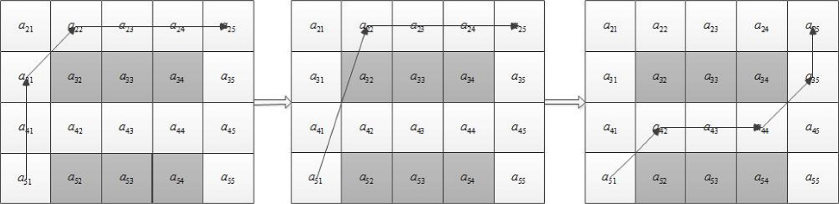
In Figure 6 (a), a random mutation is described; 7 (b) is the mutation operator mentioned in-text; and (c) is the mutation method proposed in this paper.

In Figure 6 (c), a path is $p_{i} = (a_{31}, a_{12}, a_{25}, a_{52}, a_{56})$ , a grid $a_{25}$ is selected as a mutation point, and its two adjacent path points are $a_{12}$ and $a_{52}$ . Grids $V_{1} = {a_{12}, a_{13}, a_{24}, a_{25}}$ are crossed by a path segment $a_{12} \to a_{25}$ . Grids $V_{2} = {a_{25}, a_{34}, a_{43}, a_{52}}$ are crossed by a path segment $a_{25} \to a_{52}$ . Select the point $a_{13}$ from V₁ and insert it into the chromosome. Select the point $a_{43}$ from $V_{2}$ and insert it into the chromosome. After deleting the path waypoint $a_{25}$ from the path, a new path is $p_{i}' = (a_{31}, a_{12}, a_{13}, a_{43}, a_{52}, a_{56})$ . This is one of the mutation methods in this paper.

This mutation method is different from other studies’ representations. Firstly, this function selects three waypoints, instead of selecting one waypoint, which increases the velocity of convergence; secondly, this function traverses grids crossed by path segments, such that more grids can be selected as new waypoints and guarantee that the best waypoints are obtained; and thirdly, this function can avoid obstacles and shorten the computing time.

This method is different from that in [25], with the difference being that this method can find an appropriate path point in the neighbourhood, rather than on a pathway, thereby avoiding local optimum. The theoretical basis of this operation can be interpreted in terms of geometric language, which states that the sum of any two sides of a triangle is greater than the third side.

3.7. Additional mutation

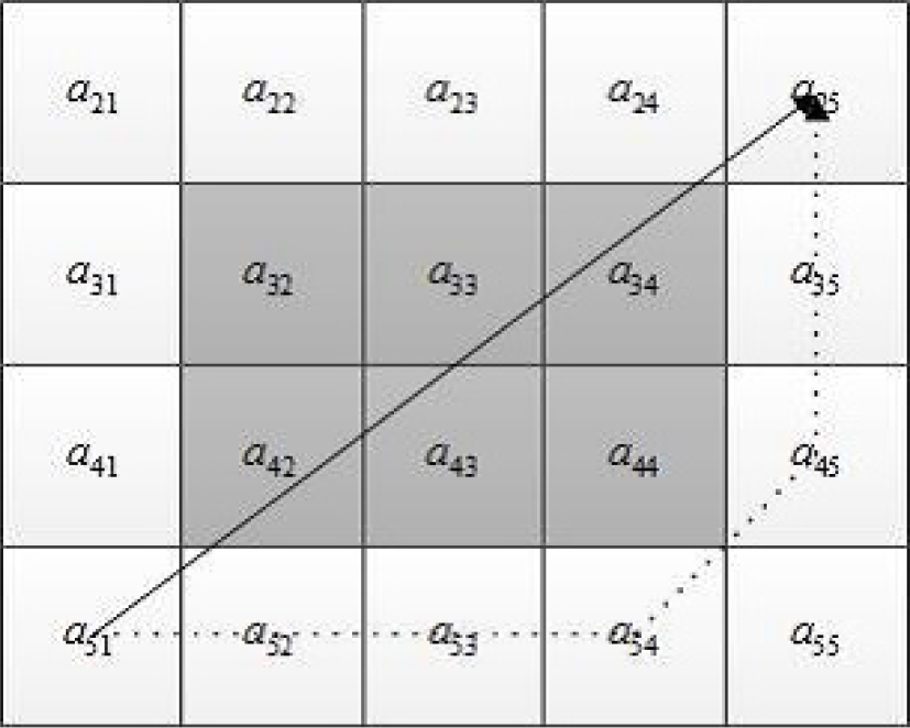
To avoid local convergence, an additional mutation operator is proposed in this study. The main idea of this mutation operation is to delete one path waypoint from a chromosome. The operation may cause intersection with obstacles. This additional mutation can increase diversity of population. Figure 7 shows how this additional mutation works.

In Figure 7, waypoint $a_{31}$ is deleted, while line segment $a_{51} \to a_{22}$ intersects with obstacle $O_{1} = {a_{32}, a_{33}, a_{34}}$ . An effective modification method is shown in section 3.8. The final path is $a_{51} \to a_{42} \to a_{44} \to a_{35} \to a_{25}$ .

Figure 7.

Comparison of mutation operators

Table 8 shows the steps of an additional mutation operator.

Table 8.

Additional mutation operation

Step	Operation
1	Selecting a way-point from chromosome marked as P_d, which is neither a starting point nor a target point, and its two neighbors are P_a and P_b .
2	The point P_d should be deleted from the chromosome.
3	Connect the point P_a and the point P_b, marked as L .
4	If the line L intersects obstacles, the chromosome should be modified and the method is in section 3.8.
5	The final path can be obtained.

3.8. Infeasible gene modification method

After crossover or additional mutation, an infeasible gene may exist in a chromosome. But this situation only appears at the genetic operation point. The method to modify an infeasible chromosome only needs to amend genes at the genetic operation point. The function is shown in Figure 8 and the steps are in Table 9.

In Figure 8, path segment $a_{51} \to a_{15}$ intersects with an obstacle. Selecting one grid from the visible space of point $a_{51}$ (for example, $a_{54}$ ) and segment $a_{54} \to a_{15}$ still intersects the obstacle. Meanwhile, another grid in the visible space of point $a_{54}$ needs to be selected, for example $a_{45}$ ; this time, $a_{45} \to a_{15}$ is feasible and a new path segment is obtained.

Table 9.

Method to modify a genetic operation, which is infeasible

Step	Operation
1	Selecting the genetic operation points and recording as P₁,P₂. P₁ is in front of P₂ in this chromosome.
2	The visible space of way-point P₁ is V_i.
4	If P₂∉V_i, means that this chromosome needs to be modified.
5	A grid P^v_m(v=1,2,…) in V_i shall be selected.
6	Setting P₁=P^v_m, and continue step 2 until P₂∈V_i.

Figure 8.

Method to modify an infeasible chromosome

Up to now, each chromosome in a population satisfies the condition of constraint and obstacle avoidance.

4. Simulation

In order to demonstrate the efficiency of the proposed algorithm, the results of three different obstacle environments are compared with other IGA studies. A hundred trials have been separately carried out in nine environments. The parameters of GA in this study are as follows:

p_{c} = 1, p_{m c} = 0.2, p_{m a} = 0.1, P o p u l a t i o n = 60, g e n e r a t i o n = 100.

where $p_{c}$ is the crossover probability, $p_{m c}$ is the conventional mutation probability, $p_{m a}$ is the additional mutation probability, $P o p u l a t i o n$ is the population size and $g e n e r a t i o n$ is the iteration number.

4.1. Simulation results in a static environment

Simulations results in six different static maps are compared with other two IGAs. Each map consists of a 16×16 grid. To evaluate the efficiency of the proposed IGA, two performance metrics were assessed: the path length and the convergence generations. The path length can represent the shortest path obtained by algorithm. The convergence generation can represent the population diversity.

The six different maps are illustrated in Figure 9.

Figure 9.

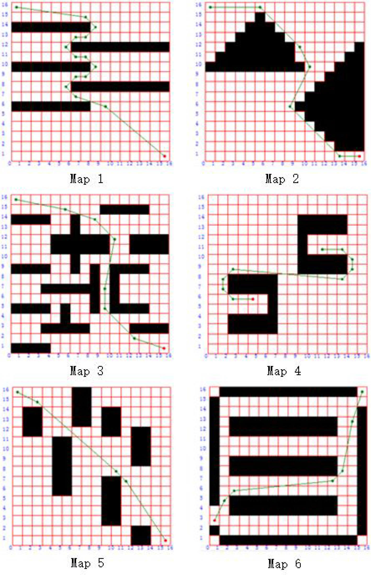
The trajectory of the best path obtained by the proposed IGA

Table 10.

Comparison of the best path according to the proposed IGA, the IGA in reference [2] and the IGA in reference [26]

Algorithm	Map1	Map2	Map3	Map4	Map5	Map6
IGA in Reference [2]	37.19	27.04	25.96	24.46	21.49	24.01
IGA in reference[26]	33.85	26.75	25.74	23.29	21.49	23.51
This paper proposed	32.36	26.44	25.59	22.70	21.49	23.38

Figure 10.

Distribution of box plot generations for each map according to different IGAs

According to Table 10, the IGA in reference [26] obtains a shorter path than that in reference [2], while the proposed IGA obtains the best performance. The reason is that the proposed IGA adopts new waypoints from the neighbourhood of two adjacent path lines, resulting in a much higher likelihood for obtaining globally optimal solutions.

Figure 10 shows the box plot of the convergence generations and the different maps for each IGA, in which each map for each algorithm is repeated 20 times. In Figure 10(a), the results of an IGA in reference [2] on Map 1 show that a maximum convergence generation is 74 and a minimum convergence generation is 23. On Map 3, we can see the lowest generation value is 15, which constitutes a premature convergence explained by a lack of diversity in the population. In Figure 10(b), the results show that the IGA in reference [26] has a large convergence distribution, while the convergence is worse than the IGA in reference [2]. In Figure 10(c), the convergence is stable on each map, with the maximum difference (19) found on Map 3. The most convergent generations are less than 25.

Simulation results on two large-scale maps are compared with A* and D* algorithms: one map consists of a 200×200 grid in Figure 11, while another one consists of a 1000×1000 grid in Figure 12. Three performance metrics are: the path length, the calculation time and the number of waypoints. The results are as follows:

Figure 11.

(a) The trajectory of the best path obtained by A*; (b) the trajectory of the best path obtained by D*; and (c) the trajectory of the best path obtained by the proposed IGA (scale 200 × 200)

Figure 12.

(a) The trajectory of the best path obtained by A*; (b) the trajectory of the best path obtained by D*; and (c) the trajectory of the best path obtained by the proposed IGA (scale 1,000 × 1,000)

Table 11.

Comparison of results according to A*, D* and the proposed IGA

Algorithm	Map with 200×200			Map with 1000×1000
Algorithm	length	time	Path point	length	time	Path point
A* algorithm	337.08	18.64	287	3378.01	65591	1821
D*algorithm	338.90	60.42	287	1763.69	1540.81	1599
This paper	329.75	16.53	10	1645.65	809.28	4

As shown in Figure 11 and Table 11, a map with the size200×200 is presented. The results indicate that A* and D* algorithms obtain optimal solutions rapidly, but the only drawback is that too many path points are stored; meanwhile, the proposed algorithm can obtain a shorter path in less time and with fewer path points.

In Figure 12, the A* algorithm takes more than 18 hours to obtain the optimized path, but the path has many jagged lines, which can cause more abrasion to the mechanics of the MR. The D* algorithm results in a shorter path than A* in less time. The proposed algorithm offers the best solution and in an acceptable time.

The only drawback of the proposed algorithm is that the time consumption is larger than A* and D* in small-scale maps. The reason is that the GA involves an optimization process based on population, while the total time is larger than A* and D* after the optimization operation. If the optimization operations are not applied, the time is almost the same for the A* and D* algorithms, while each chromosome in a population can be used as a path without considering its length.

4.2. Simulation results in a dynamic environment

In this section, simulation results obtained by the proposed IGA and the other two IGAs in three different dynamic environments are compared.

Figure 13 illustrates an initial static environment, which consists of 16 × 16 grids, and six obstacle regions formed by 57 grids [2]. Figure 14 shows a dynamic environment, which is changed after a robot moves to the third path waypoint.

Figure 13.

Referenced static environments

Figure 14.

Referenced dynamic environments

As Figures 13 and 14 illustrate, this algorithm can obtain a global optimal solution and performs better than other algorithms found in [2, 26].

In Table 12, this method converges towards the global optimal solution within 100 trials, and with less time consumed. The reason is that a concept of visible space is applied in this proposed method, such that every path waypoint only depends on its previous waypoint.

In Table 13, an optimal solution is found in 76 trials, while an approximate optimum is found in 24 trials; as such, the result is obviously better than in the literature. The time consumed is a little greater than in the literature. It is important to note, however, that the solution time contains the time consumed to handle infeasible paths.

Table 12.

Comparison of experimental results for the static environment in Figure 13

Function	IGA in Reference [2]	IGA in Reference [26]	This study
Number of optimal solutions	26	9	100
Number of near optimal solutions	70	91	0
Number of infeasible solutions	4	0	0
Value of the best fitness	27.23	27.23	27.23
Convergence generations	16	32	14
Solution time (s)	1.21	2.36	0.81
Initial solution time	0.79	0.92	0.32

Table 13.

Comparison of experimental results for the modified environment in Figure 14

Function	IGA in Reference [2]	IGA in Reference [26]	This study
Number of optimal solutions	9	27	76
Number of near optimal solutions	91	63	24
Number of infeasible solutions	0	0	0
Value of the best fitness	28.75	28.75	28.57
Convergence generations	9	22	9
Solution time (s)	0.73	1.51	0.98

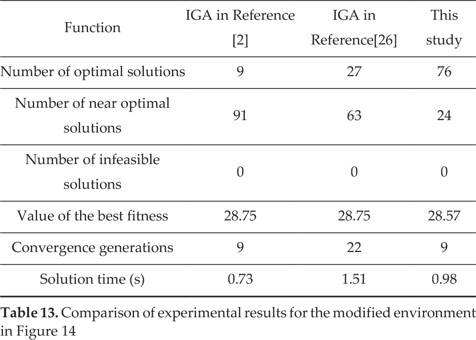
As Tables 12 and 13 illustrates, convergence results of different methods are compared. When an environment changes, both methods can converge rapidly, but this proposed method can converge towards a global optimal solution.

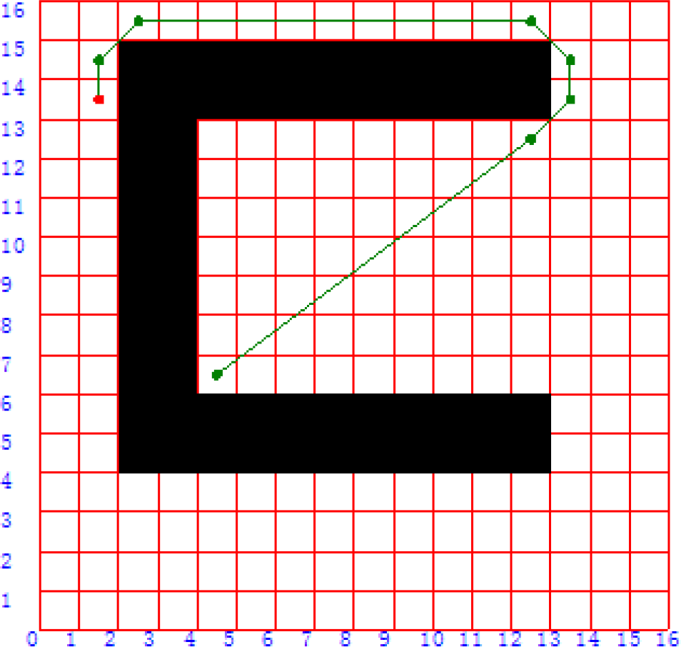
Another obstacle environment stated in [2] and [26]. Figure 15 shows a path that is found in a static environment. In Figure 16, an environment is changed after a robot moves to the fifth path waypoint.

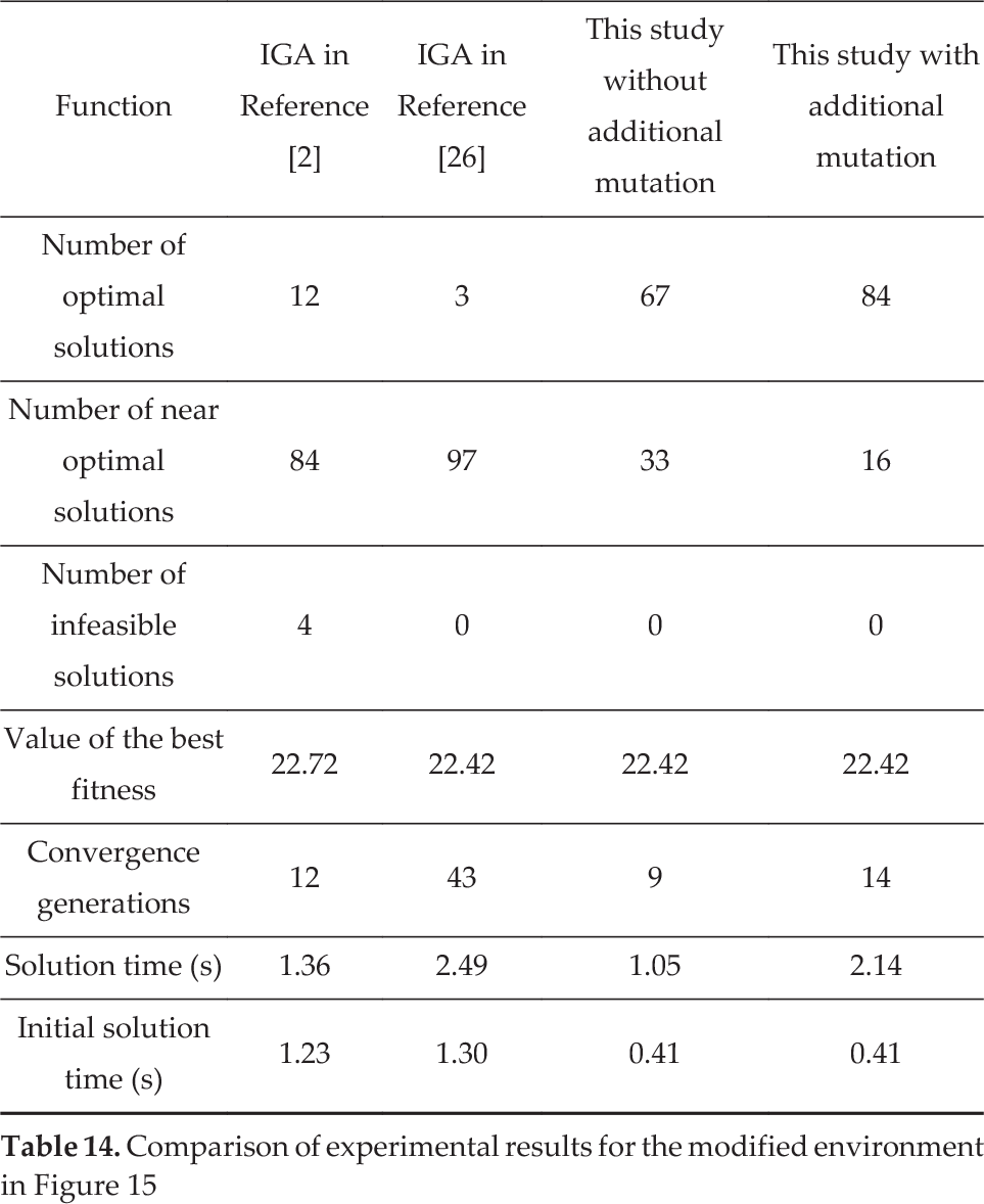
In this experiment, as shown in Tables 14 and 15, results are compared not only with reference to the literature, but also with mutation operators in this study.

In a static environment, the optimal solution is obtained in 67 trials without additional mutation, while the optimal solution is obtained in 84 trials with additional mutation and the convergence generations, while the time consumed is a little more. The initial solution time, however, is less than the method in reference [2]. The method with an additional mutation operation consumes more time, but the convergence rate is improved.

In a dynamic environment, the optimal solution is obtained in 67 trials without additional mutation, while the optimal solution is obtained in 84 trials with additional mutation. Meanwhile, both mutation methods converge in the first generation, with more speed than stated in reference [2].

As Table 15 illustrates, the method in this study converges towards the optimal solution more rapidly than in the aforementioned reference when the environment changes.

Figure 15.

Referenced static environments

Figure 16.

Referenced dynamic environments

Table 14.

Comparison of experimental results for the modified environment in Figure 15

Function	IGA in Reference [2]	IGA in Reference [26]	This study without additional mutation	This study with additional mutation
Number of optimal solutions	12	3	67	84
Number of near optimal solutions	84	97	33	16
Number of infeasible solutions	4	0	0	0
Value of the best fitness	22.72	22.42	22.42	22.42
Convergence generations	12	43	9	14
Solution time (s)	1.36	2.49	1.05	2.14
Initial solution time (s)	1.23	1.30	0.41	0.41

Table 15.

Comparison of experimental results for the modified environment in Figure 16

Function	IGA in Reference [2]	IGA in Reference [26]	This study without additional mutation	This study with Additional mutation
Number of optimal solutions	35	5	67	84
Number of near optimal solutions	63	95	33	16
Number of infeasible solutions	2	0	0	0
Value of the best fitness	23.48	22.84	22.84	22.84
Average convergence generations	11	46	1	1
Solution time (s)	0.89	1.72	0.2	0.2

In Table 15, the optimal solution can be obtained in a dynamic environment when the optimal solution is obtained in a static environment.

This proposed method can rapidly converge towards the optimal solution. In a dynamic environment, if a path segment intersects an obstacle and its two end points are $p_{1}$ and $p_{2}$ , a path point $p_{2}'$ should be added after $p_{1}$ by using the modification method in section 3.8, while $p_{2}$ should be in the visible space of $p_{2}'$ . This is the reason why the method converges rapidly.

To clarify, the method in this study can be used in irregular shapes; a new environment is modelled in Figure 17. In Figure 18, the environment is changed when a robot is going to move and the path needs to be replanned.

In Table 16, the consumed time of the initial solution is less than that in the reference. The optimal solution can be obtained in 100 trials, while the number of average convergence generations is 9.

Figure 17.

An irregular static environment

Figure 18.

An irregular dynamic environment

Table 16.

Comparison of experimental results for the modified environment in Figure 17

Function	IGA in Reference [2]	IGA in reference [26]	This study without additional mutation
Number of optimal solutions	12	19	100
Number of near optimal solutions	85	81	0
Number of infeasible solutions	3	0	0
Value of the best fitness	26.83	26.28	26.24
Convergence generations	17	35	9
Solution time (s)	3.42	3.31	0.82
Initial solution time (s)	2.97	1.77	1.13

Table 17.

Comparison of experimental results for the modified environment in Figure 18

Function	IGA in Reference [2]	IGA in reference [26]	This study without additional mutation on	This study without additional mutation
Number of optimal solutions	7	7	76	91
Number of near optima solutions	89	93	24	9
Number of infeasible solutions	4	0	0	0
Value of the best fitness	28.96	28.40	27.86	27.86
Convergence generations	19	39	6	8
Solution time(s)	1.39	2.65	0.87	1.75

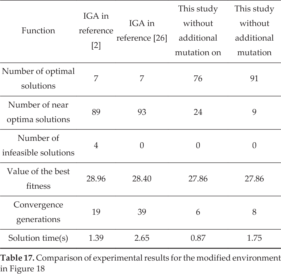
In a dynamic environment, the optimal solution can be obtained in 76 trials without additional mutation, while the optimal solution can be obtained in 91 trials with additional mutation. In Table 17, both these mutation methods can converge rapidly, but the method with additional mutation consumes more time than the other two methods.

In Table 17, the method in this study can obtain a better initial solution and faster convergence towards the optimal solution without an infeasible solution.

5. Experiments

In order to demonstrate the effectiveness of the method in this paper, experiments have been conducted.

The experiment system is divided into two parts: slave computer and host computer. The optimization algorithm was developed in the C# programming language using Microsoft Visual Studio. The program-running platform is a 2.9 GHz Intel Core Duo CPU E7500 with 2GB of memory. The slave computer is the MR, which uses uCOSII as the running system. The distance travelled is obtained from wheel odometry, while the information of the position and orientation is obtained from a GY953 AHRS module. The external dimensions of the robot are: length - 76 cm; and width - 35 cm. The results are presented in Figure 19 and Table 18.

Figure 19.

An experiment was conducted

In this system, the host computer is used to compute and send a steering order. At the beginning of the experiment, the environmental parameters – such as the size of the map, the number, shape and position of obstacles (an irregular obstacle consists of regular obstacles), the starting position and the target position – need to be put into the host computer. Moreover, the unit length of a grid is 0.8 times the width of the MR. After the optimization is completed, the host computer sends the position of the path points and the angle information to the MR via Wi-Fi.

In the dynamic environment, the environment is changed after the MR starts moving. The host computer first sends a stop command to the MR, at which the MR returns to its current position and angle value. The host computer calculates the position change of the obstacles, while the optimum results are obtained through the proposed genetic optimization algorithm. The new path results containing the position of path points and angles are sent to the MR.

In this experiment, a static environment and a dynamic environment are created in an indoor environment, in which the size of the map is 3×3m². Six obstacles are represented in the static map; in the dynamic environment, however, another obstacle is added to the map after the MR starts moving.

Table 18.

Comparison of experiment results according to three different IGAs

Algorithm	Static environment		Dynamic environment
Algorithm	Time consuming(s)	Length(m)	Time consuming(s)	Length(m)
IGA in reference [2]	31.4	2.92	46.3	3.51
IGA in reference[26]	34.7	2.92	51.2	3.39
IGA in this paper	30.5	2.92	40.1	3.14

According to Table 18, we can see that, in a static environment, the MR travels the same path, although the difference in time is huge by almost 12%. The time difference is mainly in regard to the optimization calculation and the dynamic path replanning stage.

In a dynamic environment, the length that MR moves and the time consumed are different from each other. The method in this paper obtains the shortest path and the lowest time consumption.

That said, the mechanical structure and energy consumption of the moving MR are not taken into account here. Future work will concentrate on path-smoothing with a B-spline function.

6. Conclusions

In this paper, a conventional GA was discussed and an IGA with a series of improvements was proposed, including a concept of visible space, a new encoding form and new mutation operators.

A feasible path can be obtained rapidly based on visible space. Following genetic operations, infeasible paths can be modified quickly and with a high degree of efficiency by using visible space. By using new mutation operators, the method may rapidly converge towards a global optimal solution with higher probability than other methods, not only in static environments but also in dynamic environments. An additional benefit is that a feasible path can be obtained and population diversity increased. This method is more efficient in dynamic environments because, when environment changes, only the path segments that intersect with obstacles need to be reoptimized. Compared with other algorithms, this method can reduce calculating complexity.

Footnotes

7. Acknowledgements

This work was supported in part by the Natural Science Foundation of China under Grant 61233005 and National 973 Project under Grant 2014CB744200. The author would like to thank the reviewers whose critical analysis and suggestions brought insight into the final editing of this paper.

References

Yang

. A knowledge based genetic algorithm for path planning of a mobile robot. IEEE International Conference on Robotics and Automation; 26 April to 1 May 2004; New Orleans, LA. New York: IEEE; 2004, pp. 4350–4355.

Tuncer

Yildirim

Dynamic path planning of mobile robots with improved genetic algorithm. Computers and Electrical Engineering. 2012;38(6): 1564–1572. DOI: 10.1016/j.compeleceng.2012.06.016.

Mohanta

Parhi

Patel

. Path planning strategy for autonomous mobile robot navigation using Petri-GA optimisation. Computers and Electrical Engineering. 2011;37(6):1058–1070. DOI: 10.1016/j.compeleceng.2011.07.007.

C-J

Chen

Y-H

Wong

. Path planning method design for mobile robots. Proceedings of SICE Annual Conference, 13–18 September 2011. Tokyo: IEEE; 2011, pp. 1681–1686.

Koenig

Likhachev

Furcy

Lifelong planning A*. Artificial Intelligence. 2004;155(1–2):93–146. DOI: 10.1016/j.artint.2003.12.001.

Persson

Sharf

Sampling-based A* algorithm for robot path-planning. International Journal of Robotics Research. 2014;33(13):1683–1708. DOI: 10.1177/0278364914547786.

Yazici

Kirlik

Parlaktuna

Sipahioglu

A dynamic path planning approach for multirobot sensor-based coverage considering energy constraints. IEEE Transactions on Cybernetics. 2014;44(3):305–314. DOI: 10.1109/TCYB. 2013.2253605.

Choset

Lynch

Hutchinson

Kantor

Burgard

Kavraki

Thrun

, (eds.). Principles of Robot Motion: Theory, Algorithms, and Implementation. Cambridge, MA: MIT Press; 2007, p. 632.

Zavlangas

Tzafestas

. Motion control for mobile robot obstacle avoidance and navigation: A fuzzy logic-based approach. Systems Analysis, Modeling, Simulation. 2003;43(12):1625–1637. DOI: 10.1080/0232929032000115100

10.

Hongwei

Lifang

. Research of biogeography particle swarm optimization for robot path planning. Neurocomputing. 2015;148(2015):91–99. DOI: 10.1016/j.neucom.2012.07.060

11.

Kang

B-Y

Lee

Kim

D-W

. ROBIL: Robot path planning based on PBIL algorithm. International Journal of Advanced Robotic Systems. 2014;11(47):1–14. DOI: 10.5772/58872

12.

Wang

J-F

Fan

X-L

Ding

. An improved ant colony optimization approach for optimization of process planning. Scientific World Journal. 2014;2014:294513. DOI: 10.1155/2014/294513

13.

Miao

Tian

Y-C

. Dynamic robot path planning using an enhanced simulated annealing approach. Applied Mathematics and Computation. 2013;222(2013):420–437. DOI: 10.1016/j.amc. 2013.07.022

14.

Arambula

Padilla Castaneda

. Autonomous robot navigation using adaptive potential fields. Mathematical and Computer Modelling. 2004;40(9–20):1141–1156. DOI: 10.1016/j.mcm. 2004.05.001.

15.

Rimon

Doditschek

. Exact robot navigation using artificial potential fields. IEEE Transactions on Robotics and Automation. 1992;8(5):501–518. DOI: 10.1109/70.163777.

16.

Holland

. Adaptation in Natural and Artificial Systems. Cambridge, MA: MIT Press; 1992, p. 211.

17.

Dai

Yang Yu Li

Bi-direction quantum crossover-based clonal selection algorithm and its applications. Expert Systems with Applications. 2014;41(16):7248–7258. DOI: 10.1016/j.eswa.2014.05.053.

18.

Wang

C-Y

Hwang

R-H

Ting

C-K.

UbiPaPaGo: Context-aware path planning. Expert Systems with Applications. 2011;38(4):4150–4161. DOI: 10.1016/j.eswa.2010.09.077.

19.

Shi

Cui

Dynamic path planning for mobile robot based on genetic algorithm in unknown environment. Chinese Control and Decision Conference (CCDC); 26 to 28 May 2010; Xuzhou, People's Republic of China. New York: IEEE; 2010, pp. 4325–4329. DOI: 10.1109/CCDC.2010.5498349.

20.

Al-Taharwa

Sheta

Al-Weshah

A mobile robot path planning using genetic algorithm in static environment. Journal of Computer Science. 2008;4(4):341–344. DOI: 10.1.1.165.9531.

21.

Tsai

C-C

Huang

H-C

Chan

C-K.

Parallel elite genetic algorithm and its application to global path planning for autonomous robot navigation. IEEE Transactions on Industrial Electronics. 2011;58(10): 4813–4821. DOI: 10.1109/TIE.2011.2109332.

22.

Chaari

Koubaa

Trigui

Bennaceur

Ammar

Al-Shalfan

SmartPATH: An efficient hybrid ACO-GA algorithm for solving the global path planning problem of mobile robots. International Journal of Advanced Robotic System. 2014;11(94):1–15. DOI: 10.5772/58543.

23.

Goldberg

. Genetic Algorithms in Search, Optimization and Machine Learning. 13th edition. Boston, MA: Addison-Wesley Professional; 1989, p. 432.

24.

Gelenbe

Liu

Lainé

Genetic algorithms for route discovery. IEEE Transactions on Systems, Man, and Cybernetics. 2006;36(6):1247–1254. DOI: 10.1109/TSMCB.2006.873213.

25.

Elshamli

Abdullah

Areibi

Genetic algorithm for dynamic path planning. Canadian Conference on Electrical and Computer Engineering; 2–5 May 2004. New York: IEEE; 2004, pp. 677–680. DOI: 10.1109/CCECE.2004.1345203.

26.

Karami

Hasanzadeh

An adaptive genetic algorithm for robot motion planning in 2D complex environments. Computers and Electrical Engineering. 2015;43:317–329. DOI: 10.1016/j.compeleceng.2014.12.014.

27.

Delling

Sanders

Schultes

Wagner

Engineering route planning algorithms. Algorithmics of Large and Complex Networks: Design, Analysis, and Simulation. Springer. 2009;117–139. DOI: 10.1007/978-3-642-02094-0_7.

28.

Dechter

Judea

Generalized best-first search strategies and the optimality of A*. Journal of the ACM. 1985;32 (3): 505–536. DOI: 10.1145/3828.3830.

29.

Ramalingam

Reps

An incremental algorithm for a generalization of the shortest-path problem. Journal of Algorithms. 1996; 21: 267–305. DOI: 10.1006/jagm.1996.0046.

30.

Stentz

Optimal and efficient path planning for partially-known environments. Proceedings of the International Conference on Robotics and Automation. 1994;3310–3317, CiteSeerX: 10.1.1.15.3683.

31.