Sage Journals: Discover world-class research

Abstract

Obstacle avoidance methods require knowledge of the distance between a mobile robot and obstacles in the environment. However, in stochastic environments, distance determination is difficult because objects have position uncertainty. The purpose of this paper is to determine the distance between a robot and obstacles represented by probability distributions. Distance determination for obstacle avoidance should consider position uncertainty, computational cost and collision probability. The proposed method considers all of these conditions, unlike conventional methods. It determines the obstacle region using the collision probability density threshold. Furthermore, it defines a minimum distance function to the boundary of the obstacle region with a Lagrange multiplier method. Finally, it computes the distance numerically. Simulations were executed in order to compare the performance of the distance determination methods. Our method demonstrated a faster and more accurate performance than conventional methods. It may help overcome position uncertainty issues pertaining to obstacle avoidance, such as low accuracy sensors, environments with poor visibility or unpredictable obstacle motion.

Keywords

Distance Determination Position Uncertainty Obstacle Avoidance

1. Introduction

A mobile robot must be able to get to its goal location without collision. Many approaches have been proposed to achieve this. Robots are capable of moving as intended with the positions of the robot and when the obstacles are known. However, a robot navigating an environment is subject to the measurement noise of the environment. Thus, the robot has to estimate the relative position of obstacles using the probabilistic sensor model.

The collision probability distribution is related to the position covariance [1]. However, the collision probability distribution has no boundary, meaning that the robot cannot maintain an intended distance from obstacles. Therefore, the robot should possess the ability to determine the boundary of the collision probability distribution, as well as calculate its distance from this boundary. The conventional approaches are discussed here.

The simplest approach is to calculate the distance without the position covariance. If a highly accurate measurement is available, this will facilitate a quick and easy solution. However, the position covariance depends on the environment. In addition, obstacle motion prediction increases the covariance [2]. Therefore, an alternative approach is needed in order to consider position uncertainty.

The second approach is to consider the collision probability distribution using the occupancy grid [3–4]. The obstacles are represented in an occupancy grid, while the distance to an obstacle is the distance to the nearest occupied grid unit. The occupancy grid approach takes position uncertainty into consideration, unlike the first approach. However, the occupancy grid approach requires a long computation time. The computation time is increased alongside increasing resolution of the grid.

The third technique is the error ellipsoid approach [5]. The error ellipsoid is the confidence region of a normal distribution. A mobile robot can determine the distance to an obstacle by considering the error ellipsoid. However, the error ellipsoid approach has only statistical significance [6–7]. There is no physical meaning, such as distance or collision probability. Even the conventional method of calculating the distance to the ellipsoid only considers the Lagrange multiplier error [8].

These approaches are not suitable for determining the distance of the mobile robot from a given obstacle. The position uncertainty, computation time and collision probability must be considered in order to determine the distance that ensures a negligible collision probability. The mobile robot can avoid collision in a stochastic environment using the suitable distance determination method.

In this paper, we propose a method to determine the distance that satisfies the above conditions. The proposed method consists of two steps. First, the obstacle region is determined by a collision probability density threshold. The distance function to the obstacle region is defined using the Lagrange multiplier method. Second, the solution is computed by a root-finding algorithm. The proposed algorithm can be easily applied to conventional collision-free path planning methods.

This paper is organized as follows: section 2 defines an obstacle region, a distance function with the Lagrange multiplier and a root-finding algorithm; section 3 compares the performance of the proposed method and conventional methods using three simulations; and section 4 concludes this paper and discusses potential applications.

2. Distance Determination Algorithm for Obstacle Avoidance

Let $ℛ ~ N (r, R)$ denote the estimated position of a mobile robot, where N is the multivariate normal distribution, $r$ is the mean position vector and R is the covariance matrix. Similarly, let $Q ~ N (q, Q)$ denote the estimated position of an obstacle (see Figure 1(a)). Then, the relative collision probability distribution between ℛ and $Q$ is $N (r - q, R + Q)$ . The $N (r - q, R + Q)$ must be analysed in order to avoid collision.

Figure 1.

Obstacle region (a) Let $N ([\begin{matrix} 0.20 \\ 0.25 \end{matrix}], [\begin{matrix} 0.004 & 0.002 \\ 0.002 & 0.002 \end{matrix}])$ denote a robot position and $N ([\begin{matrix} - 0.07 \\ - 0.10 \end{matrix}], [\begin{matrix} 0.012 & - 0.003 \\ - 0.003 & 0.006 \end{matrix}])$ denote an obstacle position. (b) The relative position $[\begin{matrix} - 0.3804 \\ - 0.2252 \end{matrix}]$ is represented by a blue plus-mark and the obstacle region $E ([\begin{matrix} 0.0079 & 0 \\ 0 & 0.0161 \end{matrix}]; 10^{- 2})$ is represented by a red ellipse. The shortest distance between the relative position and the obstacle region is 0.0768 $[m]$ .

First, a new coordinate system is implemented. The eigenvector of its covariance is represented by eigendecomposition: $Q + R =$ $V S^{2} V^{T}$ , where $V = [v_{1}, \dots, v_{n}]$ is the $n \times n$ square matrix composed of eigenvectors $v_{i}$ , and $S = \underset{i}{d i a g} (σ_{i})$ is the diagonal matrix of the standard deviations σ_i. Using V as a basis set of the new coordinates, the collision probability distribution is represented by $S ~ N (0, S^{2})$ , where $0$ is the zero vector. The relative position of the robot is $s = V^{T} (r - q)$ . Then, the collision probability density between ℛ and $Q$ is the probability density of $S$ at $s$ .

The probability density of $S$ is defined for the entire workspace; the mobile robot always has non-zero collision probability. Therefore, it is impossible to move to the target point without collision probability. In this situation, the best strategy is to avoid the high collision probability region. This region is determined by a collision probability density threshold. If any position has higher probability density than the threshold, this position is included in the obstacle region. The obstacle region is defined as follows.

Definition 1. Obstacle region

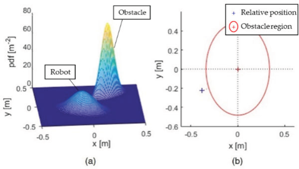
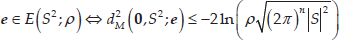
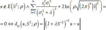
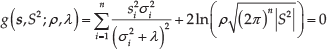
The obstacle region E is a set of relative positions, which have a greater than negligible collision probability density (see Figure 1(b)).

E (S^{2}; ρ) = {e \in ℝ^{n} : d_{M}^{2} (0, S^{2}; e) \leq - 2 ln (ρ \sqrt{{(2 π)}^{n} {| S |}^{2}})}

where ρ is the collision probability density threshold and $d_{M} (0, S^{2}; e) =$ $\sqrt{{(e - 0)}^{T} S^{- 2} (e - 0)}$ is the Mahalanobis distance [9] between $N (0, S^{2})$ and $e$ .

Let $\overset{ˉ}{E}$ denote the volume of E, where $\overset{ˉ}{E}$ is a measure of the influence of E and depends on $| S |$ and ρ (see Eq. (1)). These factors should be analysed in order to control the influence of E as intended.

Property 1.1. Volume of the obstacle region

$\overset{ˉ}{E}$ is concave down at $| S | \geq 0$ (see Figure 2 for an example) and should have a positive value. Therefore, the interval for an obstacle region to have volume is:

Figure 2.

Volume of the obstacle region (a) Assuming an obstacle is moving from left to right, its position is $(t, 0)$ , its standard deviation matrix is $[\begin{matrix} 0.5 & 0 \\ 0 & 1.9 \end{matrix}] t$ , and $ρ = 10^{- 2}$ $[m^{- 2}]$ , where t is the time. The obstacle region is a point mass at $t = 0 [s]$ . This region increases for $t \in [0, 5.855]$ and decreases for $t \in (5.855, 15.9155]$ . Finally, it disappears at $t = 15.9155 [s]$ . (b) $\overset{ˉ}{E}$ is a blue line and $\frac{\partial \overset{ˉ}{E}}{\partial | S |}$ is a red line. $\overset{ˉ}{E}$ has a positive number for $| S | \in [0, 15.9155]$ .

\overset{ˉ}{E} (S^{2}; ρ) \geq 0 \Leftrightarrow | S | \in [0, {(2 π)}^{- n / 2} ρ^{- 1}]

Proof

The boundary of E is a n -dimensional hyperellipsoid. Therefore, the following equations are established:

\overset{ˉ}{E} (S^{2}; ρ) = \frac{2}{n} \frac{π^{n / 2}}{Γ (n / 2)} | S | {(- 2 ln (ρ \sqrt{{(2 π)}^{n} {| S |}^{2}}))}^{n / 2}

(1)

\begin{matrix} \frac{\partial \overset{ˉ}{E} (S^{2}; ρ)}{\partial | S |} = - 2 \frac{π^{n / 2}}{Γ (n / 2)} {(- 2 ln (ρ \sqrt{{(2 π)}^{n} {| S |}^{2}}))}^{n / 2 - 1} + \\ + \frac{2}{n} \frac{π^{n / 2}}{Γ (n / 2)} {(- 2 ln (ρ \sqrt{{(2 π)}^{n} {| S |}^{2}}))}^{n / 2} \end{matrix}

where $Γ (n / 2) = \int_{0}^{\infty} e^{- t} t^{n / 2 - 1} d t$ is a gamma function and $\overset{ˉ}{E}$ is a positive number at the extreme point ${| S | \in [0, \infty) : \frac{\partial \overset{ˉ}{E} (S^{2}; ρ)}{\partial | S |} = 0}$ $= {(2 π)}^{- n / 2} ρ^{- 1} e^{- n / 2}$ .

\begin{array}{l} {\overset{ˉ}{E} (S^{2}; ρ) |}_{| S | = {(2 π)}^{- n / 2} ρ^{- 1} e^{- n / 2}} = \\ = \frac{2}{n} \frac{π^{n / 2}}{Γ (n / 2)} {(2 π)}^{- n / 2} ρ^{- 1} e^{- n / 2} {(- 2 ln (e^{- n / 2}))}^{n / 2} > 0, ∵ n > 0 \end{array}

(2)

There are only two points satisfying $\overset{ˉ}{E} (S^{2}; ρ) = 0$ .

{| S | \in [0, \infty) : \overset{ˉ}{E} (S^{2}; ρ) = 0} = {0, {(2 π)}^{- n / 2} ρ^{- 1}}

(3)

From Eqs. (2–3), $\overset{ˉ}{E}$ is concave down at $| S | \in [0, {(2 π)}^{- n / 2} ρ^{- 1}]$ and Property 1.1 is established.

Property 1.1 means that E disappears if the position uncertainty is too high. This property is apposite when obstacles are far enough away from the robot. However, it makes it difficult for the robot to avoid obstacles when obstacles lie near the robot. Therefore, the robot should set an alert area for which E has necessary volume. The following property pertains to the range of ρ when considering this alert area.

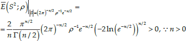
Property 1.2. Collision probability density threshold considering the alert area

E should have volume in the alert area. If $| S_{m a x} | = {max | S | :$ $o b s t a c l e i s i n$ $t h e a l e r t a r e a$ $o f t h e r o b o t}$ is known, then the proper range of ρ is:

\overset{ˉ}{E} (S^{2}; ρ) \geq 0 \Leftrightarrow ρ \in (0, {(2 π)}^{- n / 2} {| S_{m a x} |}^{- 1}]

The $| S_{m a x} |$ can be obtained from the sensor model or experimentation.

Proof

Assume that $\overset{ˉ}{E}$ is positive number when the obstacle is in the alert area. From Property 1.1,

\overset{ˉ}{E} (S^{2}; ρ) \geq 0 \Leftrightarrow | S_{A} | \leq {(2 π)}^{- n / 2} ρ^{- 1}

where S_A is the possible standard deviation matrix. The above equation is arranged as:

\overset{ˉ}{E} (S^{2}; ρ) \geq 0 \Leftrightarrow ρ \leq {(2 π)}^{- n / 2} {| S_{m a x} |}^{- 1} \leq {(2 π)}^{- n / 2} {| S_{A} |}^{- 1}

If ρ satisfies Property 1.2, then the robot can recognize the collision probability resulting from relative position uncertainty. Collision-free path planning is achieved by maintaining $s \notin E$ . The robot meets the minimum requirement in order to avoid obstacles if the distance between E and $s$ is computable. Definition 2 describes a function for calculating the distance between E and $s$ .

Definition 2. Distance considering position uncertainty

The distance calculation between ℛ and $Q$ is an optimization problem with a constraint as described below:

d_{U} (s, S^{2}; ρ) = {min ‖ e - s ‖ : e \in E (S^{2}; ρ)}

where ρ satisfies Property 1.2 (see the first paragraph of this section for notation).

If the relative position is inside of E, which is a condition that is easy to check, then the distance is zero.

Property 2.1. Inside the obstacle region

The boundary of E is a set point equal to the Mahalanobis distance of $N (0, S^{2})$ . Therefore, it is simple to distinguish what lies inside and outside of E.

d_{M}^{2} (0, S^{2}; s) \leq - 2 ln (ρ \sqrt{{(2 π)}^{n} {| S |}^{2}}) \Leftrightarrow d_{U} (s, S^{2}; ρ) = 0

Proof

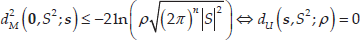
From Definition 1, points included in E have a constraint as follows:

e \in E (S^{2}; ρ) \Leftrightarrow d_{M}^{2} (0, S^{2}; e) \leq - 2 ln (ρ \sqrt{{(2 π)}^{n} {| S |}^{2}})

If $s$ has an equal constraint, there exists an $e$ that is equal to $s$ :

d_{M}^{2} (0, S^{2}; s) \leq - 2 ln (ρ \sqrt{{(2 π)}^{n} {| S |}^{2}}) \Leftrightarrow \exists e : e = s

Therefore, the minimum distance between $e$ and $s$ is zero at $e = s$ .

Property 2.1 describes the case for which the relative position is within E. However, in general, the relative position is outside of E. Therefore, the Lagrange multiplier method [10] is used to calculate d_U.

Property 2.2. Distance to the obstacle region

If the relative position is outside of E, the Lagrange multiplier method is used to find the minimum distance subject to an equality constraint. Then, d_U can be redefined using the Lagrange multiplier λ.

\begin{array}{l} s \notin E (S^{2}; ρ) \land \sum_{i = 1}^{n} \frac{s_{i}^{2} σ_{i}^{2}}{{(σ_{i}^{2} + λ)}^{2}} + 2 ln (ρ \sqrt{{(2 π)}^{n} {| S |}^{2}}) = \\ = 0 \Leftrightarrow d_{U} (s, S^{2}; ρ) = ‖ {(I + λ S^{- 2})}^{- 1} s - s ‖ \end{array}

where I is an identity matrix.

Proof

The Lagrange function corresponding to Definition 2 can be defined as:

L (e, s, S^{2}; ρ, λ) = f (e, s) + λ g (e, S^{2}; ρ)

(4)

where $f (e, s) = {‖ e - s ‖}^{2}$ is a function to be optimized, while $g (e, S^{2}; ρ) =$ $d_{M}^{2} (0, S^{2}; e) +$ $2 ln (ρ \sqrt{{(2 π)}^{n} {| S |}^{2}}) = 0$ is an equality constraint. Then, $f (e, s)$ has a minimum value when $\nabla_{e, λ} L (e, s, S^{2}; ρ, λ) = 0$ is satisfied. This equation is derived as follows:

\begin{array}{l} \nabla_{e} {{(e - s)}^{T} (e - s)} + \\ + λ \nabla_{e} {e^{T} S^{- 2} e + 2 ln (ρ \sqrt{{(2 π)}^{n} {| S |}^{2}})} = 0 \end{array}

{(e - s)}^{T} + λ e^{T} S^{- 2} = 0

e^{T} (I + λ S^{- 2}) - s^{T} = 0

e = {(I + λ S^{- 2})}^{- 1} s

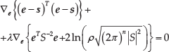
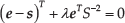
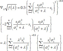
The variable $e$ in the equation g can be replaced with the above equation:

\begin{array}{l} {{(I + λ S^{- 2})}^{- 1} s}^{T} S^{- 2} {{(I + λ S^{- 2})}^{- 1} s} + \\ + 2 ln (ρ \sqrt{{(2 π)}^{n} | S^{2} |}) = 0 \end{array}

\sum_{i = 1}^{n} \frac{{{(1 + λ σ_{i}^{- 2})}^{- 1} s_{i}}^{2}}{σ_{i}^{2}} + 2 ln (ρ \sqrt{{(2 π)}^{n} | S^{2} |}) = 0

g (s, S^{2}; ρ, λ) = \sum_{i = 1}^{n} \frac{s_{i}^{2} σ_{i}^{2}}{{(σ_{i}^{2} + λ)}^{2}} + 2 ln (ρ \sqrt{{(2 π)}^{n} | S^{2} |}) = 0

(5)

Similarly,

f (s, S^{2}; λ) = ‖ {(I + λ S^{- 2})}^{- 1} s - s^{2} ‖

(6)

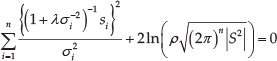
Property 2.2 is supported by Eqs. (4 –6).

Finding the closed form expression of d_U is difficult when the relative position is outside of E. Property 2.2 cannot calculate d_U directly; however, it can distinguish whether or not λ is close to the solution. Therefore, a root-finding algorithm is used in order to solve Eq. (4). The following algorithm is a process to determine the distance by implementing Properties 2.1 and 2.2.

Algorithm 1. DetermineDistance

This algorithm is the overall process used to calculate d_U and contains algorithms 2–3. Input: robot position and covariance (r, R), obstacle position and covariance (q, Q), collision probability density threshold ρ and distance error margin ε Output: distance considering position uncertainty d_u(s, S²; ρ) 01 (V, S²) ← eigenDecomposition (Q+R) 02 s ← V^T(r - q ) 03 if max_iσ_i=0 then returns ‖ s ‖ 04 if

d_{M}^{2} (0, S^{2}; s) \leq - 2 ln (ρ \sqrt{{(2 π)}^{n} | S |^{2}})

then return 0 05 [a, b] ← initializeInterval (s, S², ρ) // Algorithm 2 06 λ ← rootFinding (s, S², ρ, ε a, b) // Algorithm 3 07 return

\sqrt{f (λ)}

In lines 1-2, the relative position and covariance are calculated. If both the robot and the obstacle are point masses, then this algorithm returns a Euclidean distance (line 3). In line 4, it checks $s \in E$ using the Mahalanobis distance (see Property 2.1 for details). Finally, a root-finding algorithm is executed in lines 5-6. It searches for the λ value that satisfies $g (λ) = 0$ , where $g (λ) : =$ $g (s, S^{2}; ρ, λ)$ . The requirements for this approach are as follows:

$g (λ)$ is continuous when $λ \in [a, b]$ .

$g (a) g (b) \leq 0$

Thus, an interval $[a, b]$ satisfying conditions i and ii is required. Also, it should satisfy condition iii (see below) in order to calculate the maximum distance error.

$\sqrt{f (λ)}$ is a monotone function when $λ \in [a, b],$

where $f (λ) : =$ $f (s, S^{2}; λ)$ . When condition iii is satisfied, the maximum distance error can be calculated from end points of the interval. This value enables the root-finding algorithm to iterate until the distance error sufficiently converges to zero.

In order to satisfy conditions i-iii, the interval is inferred by $g (λ) = 0$ . This function is not differentiable at $λ = - σ_{i}^{2}$ . In other words, the maximum number of continuous subintervals is $n + 1$ : the value of g is differentiable at $λ \in (- \infty, - σ_{1}^{2}) \cup^{}$ $U_{i = 1}^{n - 1} (- σ_{i}^{2}, - σ_{i + 1}^{2}) \cup^{}$ $(- σ_{n}^{2}, \infty)$ , where $i \in [1, n - 1]$ and $σ_{i} \geq σ_{i + 1}$ . Since f has small value at $λ \to 0$ , the closest subinterval is:

λ \in (- σ_{m i n}^{2}, \infty)

(7)

where $σ_{m i n} = {min}_{i} σ_{i}$ . The upper limit of λ is derived as follows:

g (λ) \leq \sum_{i = 1}^{n} \frac{s_{i}^{2} σ_{i}^{2}}{{(σ_{m i n}^{2} + λ)}^{2}} + 2 ln (ρ \sqrt{{(2 π)}^{n} {| S |}^{2}})

0 \leq {(σ_{m i n}^{2} + λ)}^{- 2} \sum_{i = 1}^{n} s_{i}^{2} σ_{i}^{2} + 2 ln (ρ \sqrt{{(2 π)}^{n} {| S |}^{2}})

- 2 {(σ_{m i n}^{2} + λ)}^{2} ln (ρ \sqrt{{(2 π)}^{n} {| S |}^{2}}) \leq \sum_{i = 1}^{n} {(s_{i} σ_{i})}^{2}

λ \leq - σ_{m i n}^{2} + \sqrt{{(- 2 ln (ρ \sqrt{{(2 π)}^{n} {| S |}^{2}}))}^{- 1} \sum_{i = 1}^{n} {(s_{i} σ_{i})}^{2}}

(8)

From Eqs. (7–8), the interval containing a root can almost be initialized. The value of g at the end points of the interval $(- σ_{m i n}^{2}, - σ_{m i n}^{2} + \sqrt{{(- 2 ln (ρ \sqrt{{(2 π)}^{n} {| S |}^{2}}))}^{- 1} \sum_{i = 1}^{n} {(s_{i} σ_{i})}^{2}}]$ is:

lim_{λ \to λ_{min}} g (λ) = \infty

\begin{array}{l} lim_{λ \to λ_{max}} g (λ) \leq lim_{λ \to λ_{max}} \sum_{i = 1}^{n} \frac{s_{i}^{2} σ_{i}^{2}}{{(σ_{m i n}^{2} + λ)}^{2}} + \\ + 2 ln (ρ \sqrt{{(2 π)}^{n} {| S |}^{2}}) = 0 \end{array}

where $λ_{m i n} : = - σ_{m i n}^{2}$ , $λ_{m a x} : = - σ_{m i n}^{2} +$ $\sqrt{{(- 2 ln (ρ \sqrt{{(2 π)}^{n} {| S |}^{2}}))}^{- 1} \sum_{i = 1}^{n} {(s_{i} σ_{i})}^{2}}$ . Condition ii is established because $(lim_{λ \to λ_{min}} g (λ))$ $(lim_{λ \to λ_{max}} g (λ)) \leq 0$ . However, this interval does not include a lower bound, which therefore decreases the performance of the root-finding algorithm. The interval does not even satisfy condition iii. The purpose of algorithm 2 is to initialize $[a, b]$ , thereby satisfying conditions i-iii.

Algorithm 2. initializelnterval

This algorithm is a sub-algorithm of algorithm 1. It initializes the interval for the root-finding algorithm. Input: relative position and covariance (s, S²) and collision probability density threshold ρ Output: initialized interval [ a, b ] 01

a \leftarrow - σ_{m i n}^{2}

b \leftarrow - σ_{m i o}^{2} + \sqrt{{(- 2 ln (ρ \sqrt{{(2 π)}^{n} | S |^{2}}))}^{- 1} \sum_{i = 1}^{n} S_{i}^{2} σ_{i}^{2}}

03 if b < 0 then c → (a + b)/2 04 elso c ← 0 05 while g(c) < 0 06 b ← c, c ← (a+b)/2 07 return [c, b]

The above algorithm applies Eqs. (7–8) in lines 1-2 and sets the initial searching point in consideration of condition iii in lines 3-4; the initial searching point is derived from the derivative of $\sqrt{f (λ)}$ .

\begin{array}{l} \nabla_{λ} \sqrt{f (λ)} = 0.5 {\sum_{i = 1}^{n} {(\frac{s_{i} σ_{i}^{2}}{σ_{i}^{2} + λ} - s_{i})}^{2}}^{- 0.5} \\ {- 2 \sum_{i = 1}^{n} (\frac{s_{i} σ_{i}^{2}}{σ_{i}^{2} + λ} - s_{i}) \frac{s_{i} σ_{i}^{2}}{{(σ_{i}^{2} + λ)}^{2}}} \\ = λ {\sum_{i = 1}^{n} \frac{λ^{2} s_{i}^{2}}{{(σ_{i}^{2} + λ)}^{2}}}^{- 0.5} {\sum_{i = 1}^{n} \frac{s_{i}^{2} σ_{i}^{2}}{{(σ_{i}^{2} + λ)}^{3}}} \end{array}

The sign of $\nabla_{λ} \sqrt{f (λ)}$ only depends on λ because $λ > - σ_{m i n}^{2}$ . Thus $\sqrt{f (λ)}$ is monotone function at each λ interval $(- σ_{m i n}^{2}, 0]$ and $(0, \infty)$ . If $λ_{m a x} \leq 0$ , then $(λ_{m i n}, λ_{m a x}] \subset$ $(- σ_{m i n}^{2}, 0]$ , and it satisfies condition iii. Otherwise, $(λ_{m i n}, λ_{m a x}] \subset$ $(- σ_{m i n}^{2}, 0] \cup^{} (0, \infty)$ , and needs to be separated. In this case, condition iii can be achieved by setting $λ = 0$ as an initial searching point. This will be the end point of the searching interval at the next iteration.

The iteration process of algorithm 2 is simple; at each iteration, the interval is divided in two at the midpoint $c = (a + b) / 2$ . The sign of $g (c)$ is checked, the interval to satisfy condition ii is updated and the process is iterated until the lower bound is changed.

This interval initialization is in preparation for an efficient root-finding. If the interval contains both bounds, the root-finding method can use an interpolation technique, which is fast. Also, the distance function at this interval is a monotone function; therefore, the distance error bound calculation is possible with a simple computation. Algorithm 3 is the root-finding algorithm in consideration of distance error.

This algorithm is based on the Van Wijngaarden-Dekker-Brent method [11], a popular root-finding method that superlinearly converges to the root. It modifies the loop repetition condition and error criteria for considering distance error, unlike the original method [8], which considers the Lagrange multiplier error. The calculated distance error bound determines whether to repeat the loop or not. In other words, it establishes the distance error margin.

Line 3 is the loop repetition condition. If the searching point satisfies Property 2.2 or the interval has a distance error smaller than the distance error margin ε, the loop terminates. It then tries to use the fast-converging method in lines 4-6: namely, an inverse quadratic interpolation and secant method. If it fails or the result is not good, it implements a robust bisection method in lines 7-13. Lastly, it updates the interval using the search result in lines 14-17.

The determined distance computed by the proposed algorithm has two criteria: ρ and ε.

These criteria, pertaining to position uncertainty, help with improved distance determination over methods using other criteria, such as confidence [5], or the Lagrange multiplier [8]. Using the proposed algorithm, the mobile robot can compute the distance in the high collision probability region. Figure 3 shows an example of the overall process of the proposed algorithm, while a performance comparison with the conventional method is described in the next section.

Figure 3.

Process of calculating the distance between ℛ and $Q$ (a) Let $N ([\begin{matrix} 0.20 \\ 0.25 \\ - 0.05 \end{matrix}], [\begin{matrix} 0.004 & 0.002 & 0.001 \\ 0.002 & 0.002 & - 0.001 \\ 0.001 & - 0.001 & 0.003 \end{matrix}])$ denote the robot's position and $N ([\begin{matrix} - 0.07 \\ - 1.00 \\ 1.00 \end{matrix}], [\begin{matrix} 0.020 & - 0.010 & - 0.005 \\ - 0.010 & 0.010 & 0.007 \\ - 0.005 & 0.007 & 0.015 \end{matrix}])$ denote an obstacle's position. Their probability distribution is represented by the blue and red point clouds, respectively. (b) The relative position $[\begin{matrix} - 0.4477 \\ 0.0691 \\ - 0.1127 \end{matrix}]$ is represented by a blue plus-mark, while the obstacle region $E ([\begin{matrix} 0.0816 & 0 & 0 \\ 0 & 0.1274 & 0 \\ 0 & 0 & 0.1764 \end{matrix}]; 1)$ is represented by an ellipsoid. (c) A graph produced using algorithm 2 to initialize the interval. The boundaries of the interval containing a root are marked by red and blue lines. The proper initial interval $[0, 2]$ is obtained from the first iteration. (d) A graph produced using algorithm 3 to find a Lagrange multiplier for distance determination. The initialized interval is marked by red and blue lines. The results obtained after five iterations are $λ = 7.5634 \times 10^{- 3}$ , while $d_{U} = 0.2402 [m]$ . The distance error margin is $10^{- 2} [m]$ and the distance error is $0.9099 \times 10^{- 2} [m]$ .

Algorithm 3. RootFinding

This algorithm is a sub-algorithm of algorithm 1. It finds the value of λ which satisfies the constraint g(λ) = 0, or

d_{U} : = \sqrt{f (λ)}

, having a sufficiently small distance error. Input: robot position and covariance ( r, R ), obstacle position and covariance ( q, Q ), collision probability density threshold ρ, distance error margin ε, and initialized interval [ a,b ] Output: Lagrange multiplier λ 01 if | g(a) | < | g(b) |, then swap(a,b) 02 c ← a, m ← true 03 while

(g (b) \neq 0) \land (g (z) \neq 0) \land (| \sqrt{f (b)} - \sqrt{f (a)} | > ɛ)

04 if (g(a) ≠ g(b))^(g(b) ≠ g(c)) then 05

z \leftarrow \frac{{y - g (a)} {y - g (b)}}{{g (c) - g (a)} {g (c) - g (b)}} c + \frac{{y - g (b)} {y - g (c)}}{{g (a) - g (b)} {g (a) - g (c)}} a + \frac{{y - g (c)} {y - g (a)}}{{g (b) - g (c)} {g (b) - g (a)}} b

06 else

z \leftarrow b - g (b) \frac{b - a}{g (b) - g (a)}

07 if

(z \notin [(3 a + b) / 4, b]) V …

{(m = t r u e) \land (| \sqrt{f (z)} - \sqrt{f (b)} | \geq | \sqrt{f (b)} - \sqrt{f (c)} | 2)} V …

{(m = f a l s e) \land (| \sqrt{f (z)} - \sqrt{f (b)} | \geq | \sqrt{f (c)} - \sqrt{f (d)} | 2)} V …

{(m = t r u e) \land (| \sqrt{f (b)} - \sqrt{f (c)} | \geq | 2 ɛ)} V …

{(m = f a l s e) \land (| \sqrt{f (c)} - \sqrt{f (d)} | \geq | 2 ɛ)} V …

then 12 z ← (a + b)/2, m ← true 13 else m ← false 14 d ← c, c ← b 15 if g(a)g(z) < 0 then b ← z 16 else a ← z 17 if |g(a)| < |g(b)| then swap(a,b) 18 return b

3. Simulations

In this section, the proposed method is compared with conventional methods. These methods include the uncertainty determination method and the distance computation method, which use parameters listed in Table 1. The proposed method is A, while the comparison targets are B and C. The reference distance is computed by D using enough samples. The simulations are executed in MATLAB using a 2.67GHz dual-core processor.

Table 1.

Distance determination methods

	Uncertainty determination	Distance computation	Parameters used
A	Definition 1	Algorithms 1-3	Collision probability density threshold, distance error margin
B	Error ellipsoid	Bracketing method: robust implementation	Confidence, Lagrange multiplier error margin
C	Occupancy grid	Euclidean distance to the closest obstacle grid	Collision probability threshold, resolution of grids
D	Definition 1	Euclidean distance to the closest sample on the obstacle region	Collision probability density threshold, number of samples
E	Mean of distribution	Euclidean distance	−

3.1. Distance to a single obstacle

The purpose of the first simulation is to ascertain whether these methods can determine distance considering position uncertainty. The constraints of this simulation are the distance error margin $ϵ = 10^{- 2} [m]$ and the collision probability density threshold $ρ = 10^{- 2} [m^{- 2}]$ . The reference distance of D is calculated with $10^{6}$ samples on the obstacle region. In cases where these criteria are not used, the parameters are adjusted over several simulations in order to satisfy $ϵ = 10^{- 2} [m]$ and $ρ = 10^{- 2} [m^{- 2}]$ .

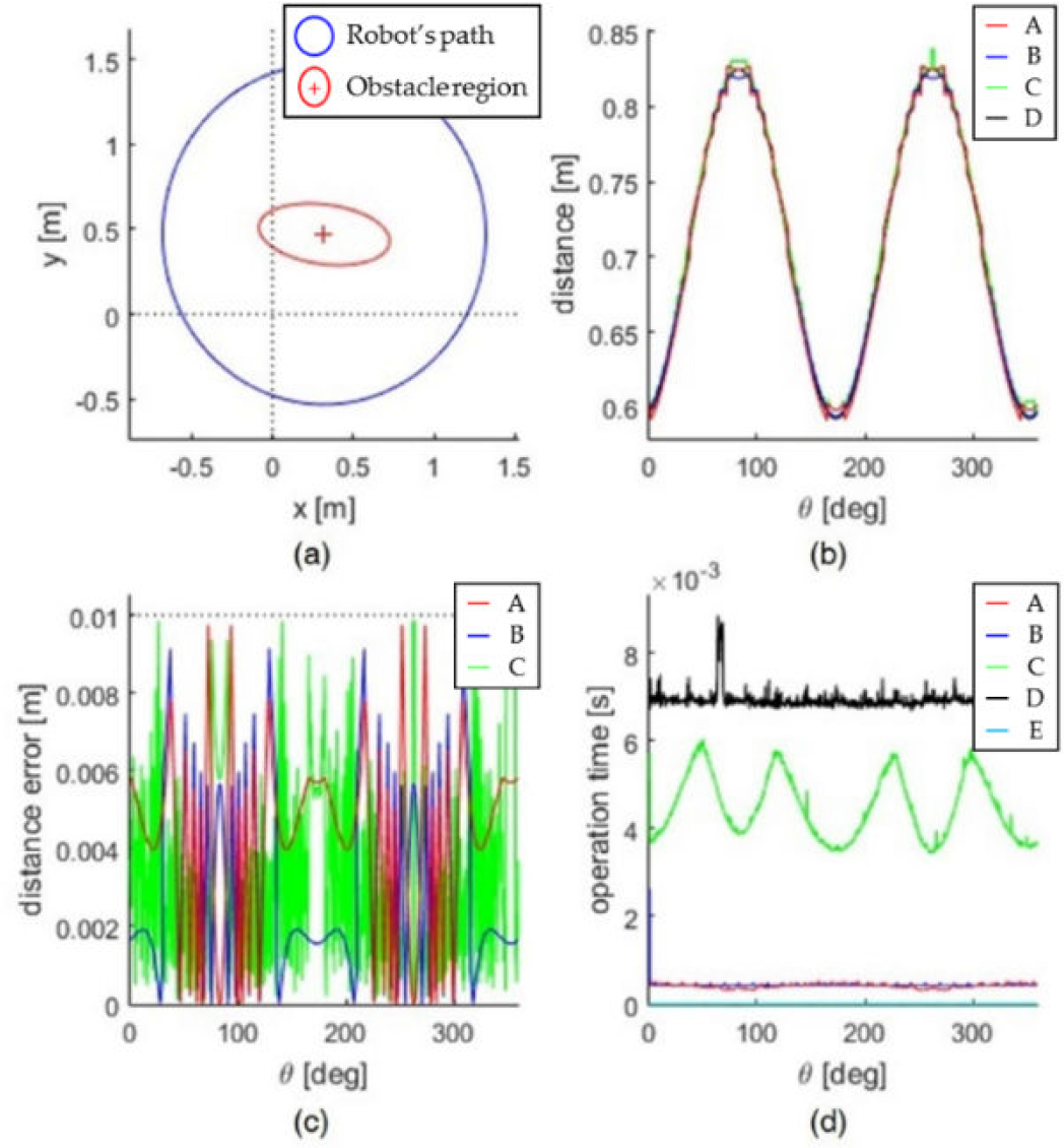
Let us consider a single static obstacle in a two-dimensional workspace (see Figure 4(a)). The mobile robot moves around the obstacle while maintaining a distance of 1 $[m]$ . B has different criteria; however, it can have the same boundary by using the confidence ${ζ : K (ζ) \approx - 2 ln (ρ \sqrt{{(2 π)}^{n} {| S |}^{2}})}$ , where $K (ζ) =$ ${k : \int_{0}^{k} \frac{t^{(n - 2) / 2} e^{- t / 2}}{2^{n / 2} Γ (n / 2)} d t = ζ}$ is the quantile function of the chi-squared distribution with n degrees of freedom and $Γ (n / 2) =$ $\int_{0}^{\infty} e^{- t} t^{n / 2 - 1} d t$ is the gamma function. Meanwhile, the grid width of C is configured by $ϵ \sqrt{2}$ to satisfy the distance error margin.

Figure 4.

First simulation: a single static obstacles in a two-dimensional workspace. Each colour in (b), (c) and (d) represent each method. A is red, B is blue, C is green, D is black and E is cyan. (a) The probability distribution of a static obstacle $N ([\begin{matrix} 0.32 \\ 0.47 \end{matrix}], [\begin{matrix} 1 & - 0.1 \\ - 0.1 & 0.2 \end{matrix}] \times 10^{- 2})$ is represented by a red ellipse and the path of the mobile robot is represented by a blue circle. The position of the mobile robot is $r = [\begin{matrix} 0.32 + cos (θ) \\ 0.47 + sin (θ) \end{matrix}]$ , where $θ \in [0, 2 π)$ is the relative angle between the robot and the obstacle. (b) Distance between the robot and the obstacle. A-D concern position uncertainty. (c) Distance error with reference to D. A-C satisfy the distance error margin of $0.01 [m]$ . (d) Operation time to determine distance. A and B show good performance.

Figure 4(b) shows the distance computed by A-D (E cannot determine distance when considering position uncertainty). The distance function of D is a sine wave, while the others are similar to a sine wave. A and B have discontinuous points if the iteration number of the root-finding algorithm is changed. C has discontinuous points if the closest obstacle grid is changed.

The distance error of A-C is represented in Figure 4(c). A and C establish the distance error to be smaller than ε. However, B requires the Lagrange multiplier error margin ε, which has no physical meaning. Thus, B cannot ensure the distance error margin. In order to satisfy ε, additional simulations are executed. The adjusted parameter $ε = 1.3 \times 10^{- 3}$ only works on simulation 1. Any change in the position probability distribution requires adjustment of this parameter.

The maximum distance error of A-C is similar to $ϵ = 10^{- 2} [m]$ (see Table 2). In this constrained situation, the operation times of A-C are represented in Figure 4(d); the proposed method A has the shortest operation time. A operates 1.05 times faster than B and 10.83 times faster than C. C is inefficient in determining the distance because the operation time of C is highly influenced by the resolution of the occupancy grid.

Table 2.

First simulation: a single static obstacle in a 2-dimensional workspace. The number of samples used in each method is 10³.

	Distance error $[m]$		Operation time $[s]$
	Mean	Max.	Mean	Std.
A	4.2862×10⁻³	9.7512×10⁻³	4.1338×10⁻⁴	4.3478×10⁻⁵

B	3.0086×10⁻³	9.1466×10⁻³	4.3246×10⁻⁴	7.0394×10⁻⁵

C	3.3317×10⁻³	9.8540×10⁻³	4.4769×10⁻³	7.2186×10⁻⁴

D	−	−	6.9301×10⁻³	2.1938×10⁻⁴

E	2.8977×10⁻¹	4.0752×10⁻¹	4.1653×10⁻⁶	6.5149×10⁻⁷

The simulation results show proposed method A to have the best performance of the methods for considering position uncertainty (A-D). The order of operation times required for distance determination is A<B≪C≪D. A and C establish the distance error margin directly; however, B requires additional process adjustments to satisfy the distance error margin. The reference method D is simple, but inefficient.

3.2. Distance to multiple obstacles

The second simulation is an extension of the first simulation: the workspace is extended to a three-dimensional space, in which multiple obstacles exist (see Figure 5(a)). Unlike the first simulation, the operation time constraint is applied. The parameters are adjusted in order for A-C to have similar operation times. This simulation reconfirms the efficiency of A-C.

Figure 5.

Second simulation: multiple static obstacles in a three-dimensional workspace. Each colour represents a different method in (b), (c) and (d). A is red, B is blue, C is green, D is black and E is cyan. (a) The seven static obstacles are represented by red ellipsoids and the path of the mobile robot is represented by a blue line. The position of the mobile robot is given by $r = [\begin{matrix} 0.32 + cos (θ) \\ 0.47 + sin (θ) \\ 0.5 cos (θ) \end{matrix}]$ , where $θ \in [0, 2 π)$ is the relative angle between the robot and the point $[\begin{matrix} 0.32 \\ 0.47 \\ 0 \end{matrix}]$ on the x-y plane. (b) Minimum distance between the robot and obstacles. The distances of A and B almost correspond with that of the reference distance. On the other hand, E does not consider position uncertainty, while the C distance appears as a stair-step function due to a lack of operation time. (c) Distance errors of A-C. (d) Function of t with respect to θ when the mean operation time of A-C is set to $6.3 \times 10^{- 4} [s]$ .

A-C compute the distance by $ρ = 10^{- 2}$ $[m^{- 3}]$ and a mean operation time of $6.3 \times 10^{- 4} [s]$ (see Figure 5(d)). To comply with this criteria, the confidence of B is calculated for each obstacle. The grid width of C is set to $ϵ_{C} \sqrt{3}$ in order to account for the three-dimensional workspace. As a result of the parameter adjustments, the distance error margin of A is $ϵ = 4 \times 10^{- 4}$ $[m]$ , the Lagrange multiplier error margin of B is $ε = 10^{- 4}$ and the grid width of C is $0.25 [m]$ .

Figure 5(b) shows the minimum distance between the robot and the obstacles. The maximum distance error of A is 3.9305×10⁻⁴ $[m]$ , which is the smallest value of all the methods. A has an accuracy 6.24 times that of B and 910.91 times that of C (see Table 3). The distance error of C depicts a stair-step function due to a lack of operation time, although the time for generating the occupancy grids is excluded.

Table 3.

Second simulation: multiple static obstacles in a 3-dimensional workspace. The number of samples is 10³ for each method.

	Distance error [m]		Operation time [s]
	Mean	Max.	Mean	Std.
A	1.3788×10⁻⁴	3.9305×10⁻⁴	6.2962×10⁻⁴	4.4104×10⁻⁵

B	6.1890×10⁻⁴	2.4526×10⁻³	6.2344×10⁻⁴	1.5706×10⁻⁵

C	1.4347×10⁻¹	3.5803×10⁻¹	6.5740×10⁻⁴	3.8015×10⁻⁵

D	−	−	5.6942×10⁻²	8.1618×10⁻⁴

E	7.4411×10⁻¹	9.2830×10⁻¹	3.5108×10⁻⁵	4.9572×10⁻⁶

B has a fundamental problem with its criteria: this method cannot ensure the distance error margin. It is difficult to determine the number of iterations for the root-finding algorithm, because the Lagrange multiplier has no physical significance. However, A ensures the distance error margin because it is capable of calculating the bounds of the distance.

The second simulation shows that A is an effective method for determining distance. This method determines apposite distance with limited operation time; the determined distance provides the maximum error within ε. However, it is still unclear whether A can help the robot to avoid obstacles. Therefore, the collision-free path planning is executed in the next simulation.

3.3. Distance determination and collision avoidance

The third simulation is used to apply distance determination methods in the context of obstacle avoidance. Let us consider a local path planner using a potential field method [12]. This path planner controls the direction of the mobile robot based on attractive and repulsive forces; the destination creates an attractive force, whereas the closest obstacle creates a repulsive force. In order to simplify the situation, this path planner only uses distance information.

Given that the base path planner cannot consider position uncertainty, its obstacle avoidance capability is dependent on the applied distance determination method. Therefore, the utility of A-E can be quantified by travel time, when the path planner is applied to A-E. A good distance determination method helps the path planner to simultaneously avoid collision and minimize the travel time.

The mobile robot should move to the goal area without collision. There exist static and dynamic obstacles, while the mean and covariance of the obstacle position are estimated (see Figure 6(a)). In order to simulate the worst case, it is assumed that the real obstacle position is a point cloud that is normally distributed. Each point in the point cloud is a position at which the obstacle may exist (see Figure 6(b)). The collision occurs when the closest point is within the radius of the mobile robot.

Figure 6.

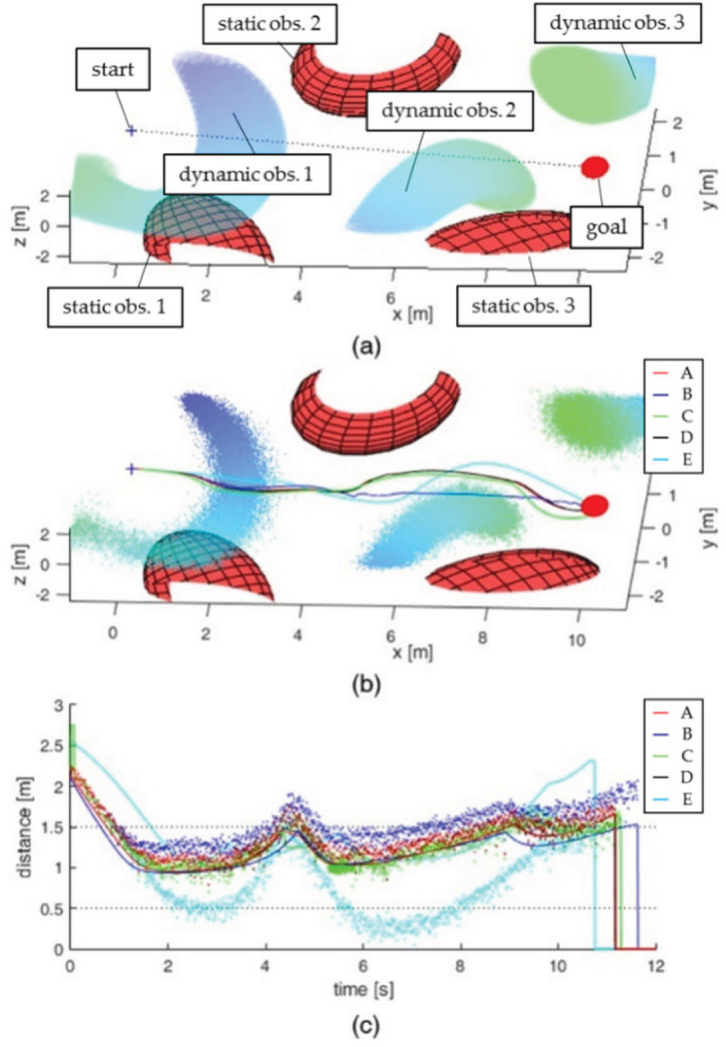
Third simulation: collision-free path planning using the potential field method in a three-dimensional workspace. Each colour represents each method in (b-d). A is red, B is blue, C is green, D is black and E is cyan. The motion of the mobile robot is planned every $0.01 [s]$ . The number of points organizing a point cloud is $10^{3}$ , while it is resampled every $0.01 [s]$ . (a) The starting point of the mobile robot $[\begin{matrix} 0 \\ 0 \\ 1 \end{matrix}]$ is represented by a blue plus-mark, while the goal point $[\begin{matrix} 10 \\ 0 \\ - 1 \end{matrix}]$ is represented by a red ball. The static obstacles are red ellipsoids and the dynamic obstacles are the ellipsoids, which change colour from blue to green depending on time $t \in [0, 12]$ . (b) The potential field method of A-E plans for collision-free paths (the paths are represented by lines). (c) The radius of the robot is $0.5 [m]$ . Its repulsive force is generated when obstacles are approached within $1 [m]$ . The determined distance is represented by lines, while the minimum distance to the point cloud is represented by points.

The five collision-free paths are generated by A-E with the parameters used in Simulation 2 (see Figure 6(b)). The distance from the closest point is depicted in Figure 6(c). The fastest path is generated by method E (see Table 4). However, it collides 283 times with point clouds because it is incapable of accounting for position uncertainty. The second fastest path is generated by method D. This method is not included in the comparison group because it is a reference with unlimited operation time.

Table 4.

Third simulation: collision-free path planning using the potential field method in a three-dimensional workspace

	Travel time [s]	Min. distance from obstacle distributions [m]		Min. distance from obstacle clouds [m]
		Min.	Mean	Min.	Mean
A	11.18	9.5339×10⁻¹	1.2657	7.8457×10⁻¹	1.3651

B	11.63	9.3384×10⁻¹	1.2248	9.8474×10⁻¹	1.5368

C	11.28	8.6603×10⁻¹	1.2838	6.9967×10⁻¹	1.3045

D	11.16	9.4926×10⁻¹	1.2670	7.9155×10⁻¹	1.3641

E	10.75	1.0524×10°	1.4684	5.4614×10⁻²	0.8713

Therefore, the fastest collision-free path is that generated by method A. The travel time error of this method is 23.5 times smaller than that of method B, and six times smaller than that of method C. In other words, proposed method A can determine a distance similar to the reference distance.

4. Experiment

This section shows a preliminary experiment on a real robot. The purpose of the robot is to move to the destination while avoiding collision with randomly distributed obstacles. Distance determination methods provide distances for preventing collisions. If the determined distance is too short, the collision probability is increased. Conversely, the robot should go around the long way. Therefore, the determined distance can be evaluated by travel time and distance to the closest obstacle.

The experiment is run in a corridor with a width of $3.0 [m]$ (see Figure 7(a)). This area randomly contains 20 cylinders. The radius of the cylinder is $0.02 [m]$ and its position is known (see Figure 7(b)). Thus, these cylinders can be used as landmarks, unlike the walls on both sides.

Figure 7.

Environment of the experiment (a). The mobile robot at the starting point (b). The map given to the robot.

The robot used in the experiment is Pioneer3dx [13]. This is a differential type of mobile robot. This robot can be assumed to be a disc with a radius of $0.2555 [m]$ . An odometer and a sonar ring are equipped, while serial communication is used to control the robot. The sonar ring consists of eight ultrasonic sensors found toward the front. Its ranging distance is $0.1 ~ 5.0 [m]$ , while its effectual angle is $30 [d e g]$ .

The localization is based on the discrete-time extended Kalman filter [14]. First, the robot pose $X = {[x y θ]}^{T}$ . is predicted by the robot model and odometer:

{\hat{X}}_{k}^{-} = f ({\hat{X}}_{k - 1}^{+}, u_{k - 1}) = {\hat{X}}_{k - 1}^{+} + [\begin{matrix} v cos θ \\ v sin θ \\ w \end{matrix}] Δ t

where $X_{0} = {[0 0 0]}^{T}$ is the initial robot pose, $Δ t = 0.1 [s]$ is the sampling time, $u = {[v w]}^{T}$ is the control input, v is the linear velocity and w is the angular velocity.

In turn, the following covariance is predicted:

P_{k}^{-} = G_{k - 1} P_{k - 1}^{+} G_{k - 1}^{T} + [\begin{matrix} {(0.0075)}^{2} & 0 & 0 \\ 0 & {(0.0075)}^{2} & 0 \\ 0 & 0 & {(0.4297)}^{2} \end{matrix}]

where $P_{0} = [\begin{matrix} {(0.01)}^{2} & 0 & 0 \\ 0 & {(0.01)}^{2} & 0 \\ 0 & 0 & {(10)}^{2} \end{matrix}]$ is the initial covariance and $G_{k - 1} = {\frac{\partial f (X, u)}{\partial X} |}_{X = X_{k - 1}^{+}, u = u_{k - 1}}$ .

Using the sonar ring and landmarks, the robot pose and covariance can be estimated as follows:

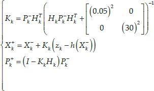
{\begin{cases} K_{k} = P_{k}^{-} H_{k}^{T} {(H_{k} P_{k}^{-} H_{k}^{T} + [\begin{matrix} {(0.05)}^{2} & 0 \\ 0 & {(30)}^{2} \end{matrix}])}^{- 1} \\ X_{k}^{+} = X_{k}^{-} + K_{k} (z_{k} - h (X_{k}^{-})) \\ P_{k}^{+} = (I - K_{k} H_{k}) P_{k}^{-} \end{cases}

where K_k is Kalman gain, $H_{k} = {\frac{\partial h (X)}{\partial X} |}_{X = X_{k}^{-}}$ , $h (X) =$ $[\begin{matrix} d i s t a n c e_{s e n s o r}^{l a n d m a r k} - R a d i u s_{l a n d m a r k} \\ a n g l e_{s e n s o r}^{l a n d m a r k} - θ_{k}^{-} \end{matrix}]$ , and z_k is the measurement of the sonar ring.

$X_{k}^{+}$ and $P_{k}^{+}$ are used to determine distance to the closest obstacle. When the distance is determined, the robot motion planner, namely the potential field method [12], can calculate the potential function. The gradient of the potential function is $z_{k + 1}$ . Therefore, the robot moves to the goal while avoiding obstacle regions.

Figure 8 shows the estimated position and real path of the mobile robot. The position uncertainty is represented by an ellipse, while the real path is in the expected range. However, E is the only method that does not consider the position uncertainty. Rather, it collides with an obstacle (see (5.3, 0.5) at Figure 8(d)). When colliding with an obstacle, the determined distance to the obstacle is $0.0916 [m]$ . The robot did not recognize the collision after it took place.

Figure 8.

Experiment: obstacle avoidance in the corridor (a) Using A, the robot has arrived at the goal without collision. (b) The path of B is similar to the path of A. (c) C shows the unstable path caused by discretely determined distance. (d) The robot collides with an obstacle, because E does not consider the position uncertainty.

The path of C is unstable. This phenomenon is caused by a discretely determined distance. In particular, (0.94, −0.17) and (5.75, −0.02) at Figure 8(c) show sudden turns. Indeed, it may generate a larger accident. Although the robot can overcome by reducing the width of the grid, the computation time will be increased.

See Table 5. A proposes the mean distance margin of $0.1071 [m]$ . This distance prevents collisions caused by position uncertainty. Furthermore, it has the shortest travel time and the shortest operation time. Although the paths of A and B are similar (see Figure 8(a-b)), B is less efficient than A, given that this experiment uses the same parameters of Simulation 1, while the size of the covariance is changed.

Table 5.

Third simulation: collision-free path planning using the potential field method in a three-dimensional workspace

	Total travel time [s]	Mean operation time [s]	Mean Determined distance to the closest obstacle [m]	Real distance to the closest obstacle [m]
	Total travel time [s]	Mean operation time [s]	Mean Determined distance to the closest obstacle [m]	Mean	Min.
A	36.70	5.7246×10⁻⁴	0.1475	0.2546	0.0705

B	37.90	6.4931×10⁻⁴	0.1521	0.2725	0.0788

C	40.30	9.1053×10⁻³	0.2471	0.2521	0.0021

E	−	2.5141×10⁻⁵	0.2285	0.2221	0.0000

5. Discussion

The proper distance determination method for collision-free path planning should consider position uncertainty, operation time and collision probability. However, conventional methods do not satisfy all these conditions. Thus, we propose a method that addresses all of these conditions in order to help obstacle avoidance of mobile robots. Simulations and an experiment were executed in order to compare the performance of the proposed method A and the conventional methods B-E (see Table 1).

Method E is the simplest and fastest method; however, this method does not consider position uncertainty. It results in collision, especially if the robot is in a highly uncertain environment; this is the only method that resulted in collision with obstacles. On the other hand, while D considers position uncertainty, it is incapable of determining a distance error margin. Using more samples is the only way to obtain accuracy.

Method C uses an occupancy grid. This method generates an obstacle grid using collision probabilities, which is suitable for collision-free path planning. However, this method requires too much operation time, since it calculates the distance to all of the adjacent obstacle grid units. When operated within a reasonable timeframe, the resolution is compromised, thereby making this method unsuitable.

B shows good performance and has a sufficiently short operation time. However, its confidence region has a low correlation with the collision probability. In addition, its root-finding method considers the Lagrange multiplier error, which has no physical meaning. Therefore, several parameter adjustments are required to maintain a desired distance whenever the environment is changed.

Therefore, we proposed a distance determination method. The obstacle region is defined, while the distance function is organized by a Lagrange multiplier method. In order to solve this problem effectively, the modified Van Wijngaarden-Dekker-Brent method is used. Unlike the conventional method, it is capable of determining the distance effectively.

The proposed method can prevent collisions caused by position uncertainty. The three simulations show that the proposed method is fast and robust: even if the operation time is higher than ideal, it ensures a collision-free distance by setting a distance error margin. Therefore, this method can be applied to a conventional path planner, without the burden of computation.

6. Conclusion

The purpose of this paper was to determine the distance to the normally distributed obstacle. Our method raises the obstacle avoidance performance of the robot, especially for highly uncertain environments. Simulations and an experiment showed that the proposed method achieves the purpose, regardless of environments.

This paper shows the potential field method application. However, other motion planners, such as the rapidly exploring random tree [15] and the fast marching square method [16] can use our method. In other words, it can facilitate consideration of the stochastic environment in relation to existing motion planners: the only constraint is that object position should be normally distributed. Future work shall aim to overcome this constraint.

Footnotes

7. Acknowledgements

This research was supported by Inha University.

References

Smith

Self

Cheeseman

. Estimating uncertain spatial relationships in robotics. arXiv preprint. 2013; arXiv: 1304.3111.

Du Toit

Burdick

. Robot motion planning in dynamic, uncertain environments. IEEE Transactions on Robotics. 2012, 28(1): 101–115. DOI: 10.1109/TRO.2011.2166435.

Elfes

. Occupancy grids: a stochastic spatial representation for active robot perception. arXiv preprint. 2013; arXiv: 1304.1098.

Nguyen

Michaelis

Al-Hamadi

Tornow

Meinecke

. Stereo-camera-based urban environment perception using occupancy grid and object tracking. IEEE Transactions on Intelligent Transportation Systems. 2012, 13(1): 154–165. DOI:10.1109/TITS.2011.2165705.

Ferrie

. High posterior density ellipsoids of quantum states. New Journal of Physics. 2014, 16(2):023006. DOI: 10.1088/1367–2630/16/2/023006.

Yuan

. Visualizing flow of uncertainty through analytical processes. IEEE Transactions on Visualization and Computer Graphics. 2012, 18(12): 2526–2535. DOI: 10.1109/TVCG.2012.285.

Řeháček

Mogilevtsev

Hradil

. Tomography for quantum diagnostics. New Journal of Physics. 2008, 10(4): 043022. DOI:10.1088/1367–2630/10/4/043022.

Eberly

(ed.). Geometric tools for computer graphics: distance from a point to an ellipse, an ellipsoid, or a hyperellipsoid. http://www.geometrictools.com: Geometric Tools, LLC; 2015: 20–23.

Mahalanobis

. On the generalized distance in statistics. Proceedings of the National Institute of Sciences of India. 1936, 2(1): 49–55.

10.

Lagrange

. In: Mécanique analytique. Sect. IV, vol. 2. Paris: 1811. 372–8.

11.

Brent

. An algorithm with guaranteed convergence for finding a zero of a function. Computer Journal. 1971, 14(4): 422–5.

12.

Choset

Lynch

Hutchinson

Kantor

Burgard

Kavraki

Thrun

. Potential function. In: Principles of robot motion: theory, algorithms, and implementation. MIT press; 2005; 77–104.

13.

Adept Mobile Robots. Manuals [Internet]. [Updated: 10 February 2016]. Available from: http://robots.mobilerobots.com/wiki/Manuals.

14.

Nonlinear Filtering. In: Grewal

Andrews

(eds.). Kalman Filtering (third ed.), Berlin Heidelberg: Springer; 2011. 310–1. DOI: 10.1007/978-3-642-04898-2_321.

15.

Hsu

Kindel

Latombe

Rock

. Randomized kinodynamic motion planning with moving obstacles. The International Journal of Robotics Research. 2002, 21(3): 233–255. DOI: 10.1177/027836402320556421.

16.

Garrido

Moreno

Javier

. Motion planning using fast marching squared method. In: Carbone

Gomez-Bravo

(Eds.). Motion and Operation Planning of Robotic Systems. Switzerland: Springer; 2015; 223–248. DOI: 10.1007/978-3-319-14705-5.

Distance Determination Method for Normally Distributed Obstacle Avoidance of Mobile Robots in Stochastic Environments

Abstract

Keywords

1. Introduction

2. Distance Determination Algorithm for Obstacle Avoidance

3. Simulations

3.1. Distance to a single obstacle

3.2. Distance to multiple obstacles

3.3. Distance determination and collision avoidance

4. Experiment

5. Discussion

6. Conclusion

Footnotes

7. Acknowledgements

References