
Abstract
The process of finding an optimum, smooth and feasible global path for mobile robot navigation usually involves determining the shortest polyline path, which will be subsequently smoothed to satisfy the requirements. Within this context, this paper deals with a novel roadmap algorithm for generating an optimal path in terms of Non-Uniform Rational B-Splines (NURBS) curves. The generated path is well constrained within the curvature limit by exploiting the influence of the weight parameter of NURBS and/or the control points' locations. The novelty of this paper lies in the fact that NURBS curves are not used only as a means of smoothing, but they are also involved in meeting the system's constraints via a suitable parameterization of the weights and locations of control points. The accurate parameterization of weights allows for a greater benefit to be derived from the influence and geometrical effect of this factor, which has not been well investigated in previous works. The effectiveness of the proposed algorithm is demonstrated through extensive MATLAB computer simulations.
Keywords
1. Introduction
Since the 1980s, path planning has been a hot issue in robotic and automation fields. The solution should not only guarantee a collision-free path with minimum travelling distance, but also provide a smooth and feasible path from the initial location to a goal location in an environment cluttered with obstacles. The path planning environment can be either static or dynamic. For the static environment, the whole solution can be found before starting execution. However, for dynamic or partially observable environments, replanning is required frequently and more update time is needed. There are many studies on robot path planning using various approaches, which can be broadly classified into local and global methods.
Global or deliberative approaches include classic strategies that rely on capturing the topology of the environment and synthesizing it, either in a graph (visibility graph, Voronoi diagram, cell decomposition,…), or in a tree connecting the start to the goal position (Rapidly-exploring Random Trees (RRT),…). They also include heuristic strategies (genetic algorithms, neural networks,…). Local or reactive approaches, on the other hand, can operate online, exploiting local sensor information. These approaches include, likewise, classic strategies (potential fields, dynamic window,…) and intelligent methods (fuzzy logics,…). Although the fact that local approaches can be applied in any type of environment, whether static or dynamic, the convergence towards the final position is not guaranteed. For a broader review of past research, we refer the reader to [1, 2].
The review of research works on robotic path planning shows that most of them provide a piecewise linear solution. Thus, the robot following this path has to stop and restart frequently, which causes the waste of energy. To obtain a smooth path, many curves have been introduced as path primitives. The focus is on turning a sequence of configurations into a smooth curve that is then passed to the control system of the robot. The used curves fall into two categories: those whose coordinates have a closed-form expression (B-spline, quintic polynomials, polar splines, etc.) and parametric curves whose curvature is a function of their arc length (clothoids, cubic spirals, intrinsic splines, etc.) [3].
Dubins paths, which are made by joining straight lines and circular arcs of maximum curvature, were proposed to generate feasible paths for car-like robots [4]. However, as highlighted by Fraichard and Scheuer [3], the curvature of this type of path is discontinuous. In fact, discontinuities arise at the transitions between segments and arcs, and between arcs with opposite directions of rotation. Following that, they proposed the first steering method that computes paths with continuous curvatures, upper bounded curvatures and upper bounded curvature derivatives. This method, called CC Steer, computes paths made up of line segments, circular arcs and clothoid arcs. Nevertheless, as mentioned in [5, 6], clothoids have no closed form and have to be approximated by high-order polynomials and splines, which limits their use for real-time robotic applications.
Meanwhile, Li et al. [7] have introduced a technique to derive a smooth, obstacle-avoiding curve from a given obstacle-avoiding polyline path. In fact, supposing that a planar region that contains some obstacles is given, and assuming that a polyline path that does not touch any of the obstacles is also given, the guiding polyline will be replaced by a
As a continuing work on
Maekawa et al. [11] have introduced a roadmap algorithm for generating collision-free paths in terms of cubic B-spline curves. The method employs the visibility graph technique. In fact, once the reduced visibility graph is obtained, a weighted graph is generated by considering the Euclidean distances between the endpoints as weights. Then, the shortest path is found using Dijkstra's algorithm. Since the obstacles and the boundaries of the configuration space are assumed to be polygonal, the resulting path consists of straight line segments. Therefore, in order to generate a curvature continuous path, the intersection points of the resulting line segments are interpolated using a cubic B-spline curve. However, the interpolated curve may collide with both obstacles and the boundary segments. Also, the curvature may exceed the maximum allowable value. To solve these problems, a simulated annealing method has been used. Lobaton et al. [12] have presented a method for planning curvature-constrained paths to multiple goals using circle sampling. In fact, a roadmap is constructed by sampling circles of constant curvature and then generating feasible transitions between them by providing a closed-form formula. Then, the multi-goal planning problem is formulated as finding a minimum directed Steiner tree over this generated roadmap. Greedy heuristics are introduced to reduce the exponential complexity of the problem.
Among these different curves, Non-Uniform Rational B-Spline (NURBS) curves are more intuitive due to their important properties, which will be dealt with in more detail in the next section. NURBS have a broad range of applications in various domains, but a limited use in robotics. Recently, Siddavatam et al. [13] have developed a new method of robot motion planning in a dynamic environment using offset NURBS. Their methodology, used to obtain the optimal shortest path, can be further subdivided into levels. The first level consists in obtaining the mathematical dynamic polygonal environment that models the obstacles. The second one aims to identify the obstacles found along the ideal path. The next level consists in a mathematical model that constructs a new set of optimal points to form the shortest path from the initial to the end point. The purpose of the subsequent stage represents the plotting of a newer set of points, along with taking vector additions into consideration if the two points to be joined are from different obstacles, as well as avoiding any intersecting point, if encountered. Finally, the NURBS technique is applied to plot the shortest path using the computed set of points. NURBS offset is generated for the computed shortest path in order to avoid any collision. Xidias and Aspragathos [14] have presented a new algorithm for finding the shortest continuous curvature-constrained path for a car-like robot using S-Roadmaps. Indeed, in the beginning, random samples from the 2D environment are taken and, using Delaunay triangulation, a graph is constructed. Then, after adding start and goal positions to this graph, a B-Surface concept is employed to represent the robot's environment. The second step consists in building a roadmap onto the B-Surface, one that does not incorporate any kinematical constraints. The paths encoded in the roadmap consist of poly-geodesic segments. Optimization and smoothing of these paths are provided by using NURBS curves.
As will be detailed in the next section, a NURBS curve is defined by its order, a set of weighted control points and a knot vector. Seeing that they are a weighted extension of Non-Uniform Rational B-splines, a high level of flexibility and a great capacity to produce natural smooth curves is guaranteed. Therefore, accurate parameterization is needed to meet the desirable result. This was not well-considered in previous path planning algorithms, mainly the parameterization of the weight factor that has interesting geometric and analytical interpretations.
In this paper, we address two key issues in robot path planning: path continuity and maximum curvature constraint for nonholonomic robots. Its main contributions are the following. First, the adaptivity of the proposed method, which provides the optimal or near-optimal path in terms of length and obstacle avoidance, and respects the curvature constraint related to the robot's characteristics, irrespective of the number, size and location of obstacles. Second, NURBS curves are not used only as a means of smoothing but are also involved in meeting the system's constraints via a suitable parameterization of control points' weights as well as their location. Through rigorous computer simulations, the proposed method is shown to perform excellently and gave satisfactory results.
The remaining part of this paper is organized as follows. Section 2 introduces NURBS curves. In Section 3, the problem is formulated. The details of the proposed approach are introduced in Section 4. Computer simulations are given in Section 5. In Section 6, we present a brief discussion. Finally, in Section 7, we summarize the main findings of the article.
2. Non-Uniform Rational B-Splines (NURBS) Curves' Approximation
In this section, we briefly introduce the mathematical definition of NURBS curves. In addition, we present their important characteristics that have contributed to their wide acceptance as standard tools for geometric representation and design. Then, we investigate the geometric meaning of the weight parameter.
2.1. Definition
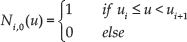
A

where

The

The knot vector
Some reasons for the widespread acceptance and popularity of NURBS in the CAD/CAM and graphics community are as follows [15]:
They offer a common mathematical form for representing and designing both standard analytic shapes and free-form curves and surfaces.
By manipulating the control points as well as the weights, NURBS provide the flexibility to design a large variety of shapes.
Evaluation is reasonably and computationally stable.
NURBS have clear geometric interpretations.
Strong convex hull property: the NURBS curve is contained in the convex hull of its control points. Moreover, if
NURBS are invariant under scaling, rotation, translation and shear as well as parallel and perspective projection.
Local modification: if a control point Pi is moved or a weight wi is changed, it will affect the curve only in
2.2. Weights parameter influence on NURBS curves
As shown above, a NURBS curve is defined by its control points, weights and knots. Therefore, modifying any of these parameters changes the curve's shape. Throughout this paper, we use the influence of the weight factor on the resulting curve. The weight of a point Pk determines its influence on the associated curve. Thus, increasing (or decreasing) wk leads to the augmentation (or diminution) of

NURBS curve approximation of
It should also be noted that a control point with a weight of zero removes the contribution of this point on the generated curve and when all weights are of unit value, the curve behaves as a non-rational B-spline. For further detail, we refer the reader to [16].
3. Problem Formulation
The problem of path planning is usually formulated as follows. Given a mobile robot moving in an environment Ω, the objective is to find a feasible path from the start position

Consequently, we denote by

We assume a circular model of the nonholonomic robot R with a diameter d, taking into account its dimensions, and a minimum radius of curvature

Formulation of the path planning problem in terms of our approach
4. Navigation Architecture
4.1. Overview
The proposed approach can be seen as the composition of two consecutive blocks: the first focuses on determining an optimal polyline path from the starting position S to the arrival T. This linear piecewise path should lie in the middle of the obstacle-free configuration, in order to increase the degree of security. It should also be of minimal length. The second focuses on the smoothing process using NURBS curves and taking into account the robot's minimum radius of curvature. An accurate parameterization of the locations of control points, as well as of their respective weights, is proposed. The final existing solution ensures the constraints of security and maximum allowable curvature. The proposed robot path-generation scheme is illustrated in Figure 3.

The schematic diagram of the proposed method
4.2. Collision-free polyline path generation
In this section, we present the steps of determining an obstacle-avoiding polyline path between the start position S and the target position T. The main idea is based on capturing the topology of the search space
We recall that skeletonization consists in reducing a form into a set of curves called ‘skeletons’, while respecting the topology of the considered form. This representation must be as thin as possible (at most, one pixel thick). It must also respect the connectivity and be centred within the shape it represents. The algorithm used in this approach is a metric criteria method [17] based on the calculation of a function that operates within a neighbourhood of eight points. The basic idea is the calculation for each image point

p(i,j) and its neighbourhood


Intuitively, the points inside the form are associated with a small value of
Sweep 1: Calculates local characteristics of each point:
Sweep 2: Either eliminates or does not eliminate the point, in terms of its characteristics.
In general, the start and goal points are not part of the skeleton (Fig. 5 (b)). Therefore, these two positions must be connected to the considered medial axis. This operation must provide a new ‘extended’ skeleton (Fig. 5 (c)) upon which the robot will progress.
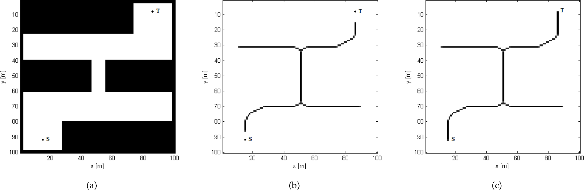
Skeletonization of an obstacle-free space: (a) the configurations space, (b) initial skeleton and (c) extended skeleton
The next step is the conversion of the extracted skeleton X into a graph, which requires the classification of pixels of X into Junction Points, End Points, Curve Points and a Critical Curve Point by using a morphological process [18]:
Thereby, the detection of interest points of X is important for a structural description that captures the topological information embedded in the skeleton. In fact, the thin lines can be converted into a weighted graph


The graph weights are generated by considering the Euclidean distances between vertices. As each edge corresponds to a corridor in which the robot may move, this last must be of a width l larger than the robot diameter d. If this is not the case, such an arc must be deleted; hence the need for the reduction step of the graph G to obtain a partial graph

The resulting graph

Graph disconnection after the reduction step

4.3. Continuous smoothing of collision-free polyline path using NURBS curves
The existing shortest path

Collision-free shortest path: (a) linear piecewise path (S opt )), (b) path smoothing using a NURBS curve
Generating a NURBS curve requires the specification of the set of control points to approximate. It must, likewise, parametrize the weights associated with this set, as well as the knot vector U. For our purposes, the control points are extracted from the selected skeleton

where

The single source shortest path (Figure 7 (a)) is smoothed following the steps already mentioned, giving the NURBS curve C, which models the planned path (Figure 7 (b)).
The previously generated NURBS curve is, in fact, a Non-Uniform Rational B-Splines curve, given that all the control points have the same weight value. We point out that two constraints must be ensured by the planned path: collision avoidance and the curvature limit related to the robot's minimum radius of curvature. Actually, the approximation of the set of control points extracted from the polyline path may distort the constraint of obstacle avoidance, since the approximated curve can introduce a large deviation relative to the determined shortest path
4.3.1. Ensuring the non-collision constraint
To ensure the security of the planned path, we investigate the influence of the weight parameter on the curve. In fact, the increase in value of wi attracts the curve towards the associated point Pi which, consequently, ensures the constraint of non-collision. The idea consists, in the first place, in localizing the set T of curve points that intersect obstacles:

To determine this set, it is sufficient to check for each point

Once the set

Collision Avoidance Process: (a) linear piecewise path (S opt )), (b) path smoothing using a NURBS curve (before the collision avoidance process), initial weights vector W=(1,1,1,1,1,1,1,1,1,1) and (c) path smoothing using a NURBS curve (after the collision-avoidance process), final weights vector W=(1,1,1,1,1,1,1,10,8,1)
4.3.2. Ensuring the curvature constraint
In the previous section, we determined a collision-free and smooth path modelled by a NURBS curve of degree p (
The curvature parameter can be matched tothe velocity and acceleration constraints. In fact, a continuous allowable curvature is of practical importance for mobile robot planning and control, because a path with a smaller variation of curvature is more appropriate for tracking and control than a path with large deviation of curvature, in order to avoid the rapid change of radial acceleration [9]. As a parametric curve, the curvature function of a NURBS curve is computed as follows [22]:

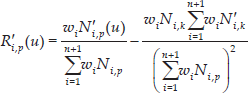
where

where:
A detailed description of the calculation of derivatives of a NURBS curve is presented in [16]. Figure 9 illustrates a NURBS curve approximation of seven control points and its associated curvature variations. The goal of this section of the path planner is to refine the previously generated curve by introducing a bounded curvature constraint:

(a) NURBS curve approximation of P1,‥,P7. (b) Associated curvature profile.

Recall that the radius of curvature is the radius absolute value of the circle tangent to the curve at the concerned point; this circle is called an osculating circle to the curve at that point. This measurement indicates the bending degree: the higher the radius of curvature, the more the path approximates a straight line and vice versa.
As shown in Section 2.2, as the weight of a control point increases, the curve comes closer and if the weight is of sufficient importance, the curve will follow closely the considered control point. We note that the weight parameter is inversely proportional to the radius of curvature. In fact, as shown in Figure 10, the gradual increase in the value of the weight of the control point Pi from 0.25 to 5 led to the progressive diminution of the radius of curvature of Qj, the closest curve point to Pi.
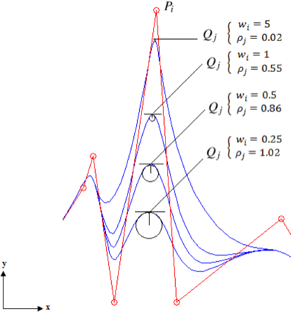
Variation weight vs. radius of curvature
Being the inverse of the radius of curvature, the value of the curvature increases with an increase in weight. Consider the example of the NURBS curve approximation of seven control points (Figure 1): the change in the weight value of
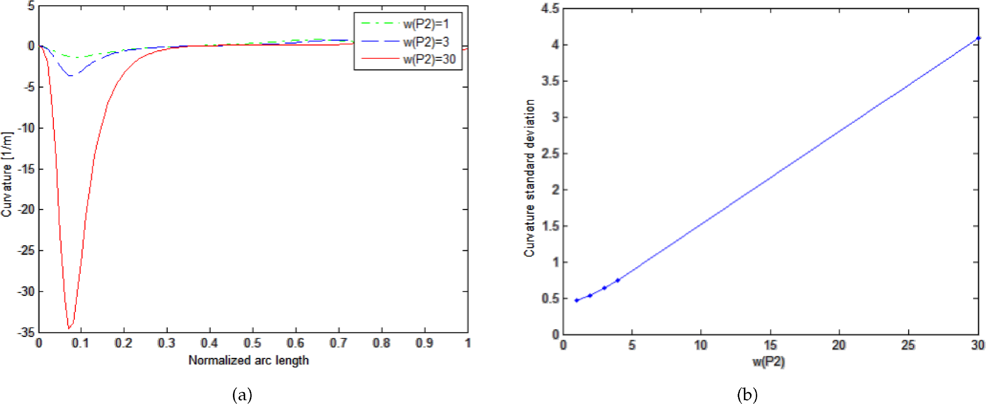
(a) Curvature profiles of the NURBS curves of Figure 1. (b) Associated variation of curvature standard deviation with P2 weight's varying.
Therefore, to readjust the generated trajectory C in response to the constraint (16), the algorithm consists, firstly, in detecting the set of curve points

The following procedure involves identifying for each component of
Figure 12 (a) illustrates the NURBS curves before (blue) and after (pink) applying the procedure of curvature correction. The blue curve is a

(a) NURBS curves before (blue) and after (pink curve) the process of curvature correction (degree = 4, number of control points = 15). (b) Associated curvature profiles (before (blue) and after (pink curve) the process of curvature correction).
For the initial curve, the two curve points that violate the curvature constraint are marked in red. To refine this path and make it eligible, the algorithm acts upon the weights of four control points (P5, P6,
For the rest of our approach, after validating the collision avoidance constraint, the algorithm checks the validity of the curvature constraint by calculating the set
5. Simulation Results
In this section, we report on extensive experiments to evaluate the effectiveness and performance of the proposed approach for global curvature-constrained path planning using NURBS curves modelling. We considered simulations under various conditions related to the configuration's space size; the number, location and size of obstacles; the start and target positions and the robot's parameters (diameter and minimum radius of curvature). Values of used input parameters are shown in Table 1, whereas Table 2 gives the experimental results for all tested configurations.
Parameters used for robot path generation

Experimental results

In Map I, after having stored the geometrical representation of the environment and after having calculated the corresponding extended skeleton (which is modelled to obtain a graph representation of all feasible paths on which a process of graph reduction is applied, keeping only those sectors that have the minimum width allowing the robot to pass through the corridor formed by the two vertices i and j), then, with the help of the Bellman Ford algorithm, a single-source shortest path, in the resulting graph, is determined. To ensure the smoothness property of the selected path, a

Initial generated path (blue curve)
The corresponding distribution of curvatures is presented in Figure 14 (b). As the constraint of minimum radius of the curvature of the robot was set at one, therefore the path must have the value of one as the maximum allowable value of curvature. This constraint was not ensured, since the corresponding curvature variations have an inflection point (the black dot in Figure 14 (b)), where the absolute curvature value exceeds the permissible value. The algorithm of curvature correction acted on the initial curve by decreasing the weight of the 4th control point and displacing P12 from the position (65,59) to (63,61).

Simulation results under MapI-1: (a) generated path before the process of curvature correction, (b) associated curvature profile (σ(curvatures)=0.20), (c) generated path after the process of curvature correction, where the associated weights vector is W=1,1,1,0.8,1,1,1,1,1,1,1,1,1 and (d) associated curvature profile (σ(curvatures)=0.17)
To prove the adaptivity of our approach, Figure 15 shows a second experiment performed in the same environment as the first one and with the same target position. The start position, robot diameter and minimum radius of curvature have been changed. As illustrated, the proposed algorithm succeed in finding the desired path.

Simulation results under MapI-2: (a) generated path before the process of curvature correction, (b) associated curvature profile (σ(curvatures)=0.19), (c) generated path after the process of curvature correction, where the associated weights vector is W=(1,1,0.8,1,1,0.7,1), and (d) associated curvature profile (σ(curvatures)=0.11)
In Map II, the proposed method has allowed us to provide, in the first step, a smooth and the shortest free-collision path (Figure 16 (a)). Then, in second one, the solution was refined by locally modifying the previously generated path (displacing the two control points, P7 and P10) so that it has a distribution of curvatures that respects the limit value allowable by the robot (Figure 16 (b)), which gives an optimal path from start to target points in the configuration space. Thus, the adopted path is modelled by a NURBS curve approximating 13 control points from S to T.
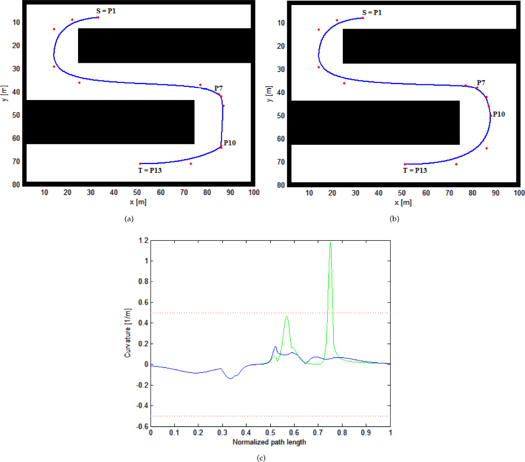
Simulation results under MapII: (a) generated path before the process of curvature correction (σ(curvatures)=0.16), (b) generated path after the process of curvature correction (σ(curvatures)=0.06) and (c) curvature profiles before (green) and after (blue) the process of curvature correction; the dotted red lines represent the curvature limit constraint
Figure 16 (c) shows the curvature profiles before (green) and after (blue) the curvature correction procedure. The maximum absolute value of curvature equals 0.17, respecting the maximum allowable value (0.5) and the standard deviation of curvatures equal to 0.06. This low value indicates that the data points tend to be very close to the mean, proving the homogeneity of the distribution of curvatures and, consequently, the smoothness criterion. Figure 17 shows the results obtained under four further different maps. All computed paths were modelled by NURBS curves, which ensures the smoothness and the curvature limit.
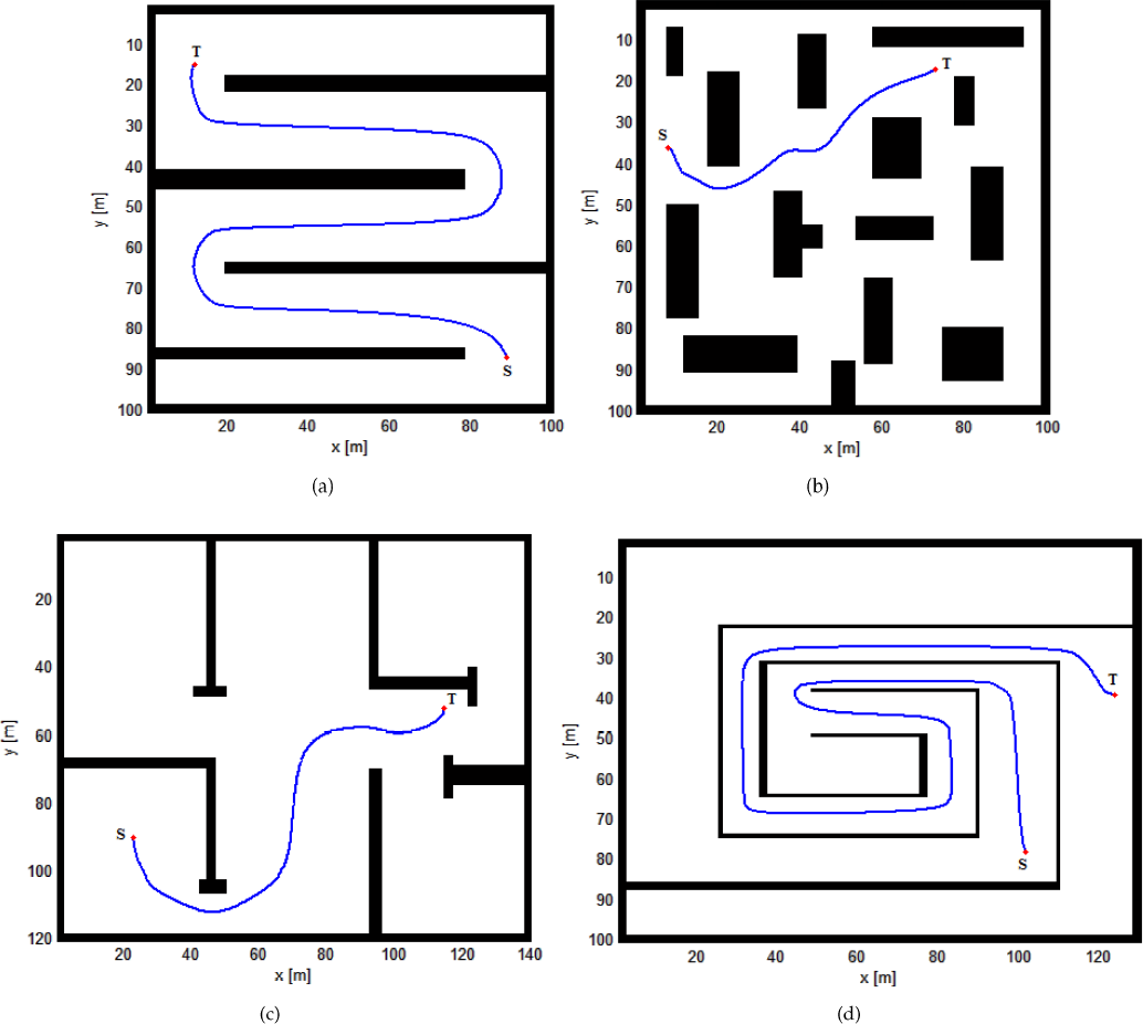
Simulation results under various maps: (a) back and forth, (b) dense, (c) rooms and (d) square spiral
6. Discussion
In this research, a novel path-planning algorithm was established and investigated using extensive simulation studies. Using this method, the robot seeks the best path to navigate safely with respect to its minimum radius of curvature.
To search for the shortest and most secure path, we applied the Bellman algorithm to the graph constructed from skeletonization of an obstacle-free space, which guarantees, therefore, a higher degree of security (obstacle avoidance), as the path to be calculated is always closest to the middle of corridors in which the robot moves. In addition, this method guarantees a shorter path length than RRT-based approaches, which produce suboptimal solutions due to the random sampling principle [10]. Compared with the algorithms described in [25, 26], our method not only ensures the smoothness property, which has been proven important in the process of robot navigation, but also respects the limit of allowable curvature. As for the methods [3, 7, 8, 9, 10, 11, 12], the proposed method is distinguished by the use of modelling with NURBS curves, which are much more flexible than other smoothing techniques, coupled with the fact that NURBS algorithms are fast and numerically stable. Moreover, our method uses varied values for the weight parameter, unlike many existing path planning methods that use NURBS curves, such as [13, 27], where all weights of control points are set at one. In [14], the weight factors associated with the nodes of the S-Roadmap are equal to three and, in this manner, it is possible to control the distance of the robot from the nodes. Consequently, by fine-turning these weights, either closer or more distant proximities can be achieved. Thereby, NURBS curves are used only in the smoothing process of the generated paths and no accurate parameterization of the weight parameter has been provided.
The major contributions of this paper are the following. First, the adaptivity of the proposed path-planning algorithm, which was able to drive the robot autonomously and to seek the best possible path to reach the target, even in complicated scenes. Indeed, it not only provides the near-optimal path in terms of length and obstacle avoidance but also respects the curvature constraint relating to the robot's characteristics and irrespective of the number, size and location of obstacles. Second, NURBS curves are not used only as a means of smoothing but they are also involved in meeting the system's constraints via a suitable parameterization of the weights of control points, which allows greater benefit to be derived from the influence and the geometrical effect of this parameter, which has not been exploited well in previous works. In addition, the control points' locations were used to control the curve shape locally, in order to satisfy the problem requirements.
7. Conclusion
In this study, we present a global curvature-constrained path planning method based on graph theory and NURBS curves. This method provides a deterministic approach for generating paths with a continuous curvature and a continuous derivative of curvature; hence, smooth paths are determined. It has been shown that the proposed algorithm is capable of efficiently finding the shortest, and a more secure, existing path, whatever the complexity of the configuration space. Nevertheless, the environment in which the robot moved was static and the information of the environment was known a priori. Future work will investigate the problem of path planning in an unknown dynamic environment. Furthermore, it will be interesting to adopt our algorithms in real-world applications.
Footnotes
8. Acknowledgements
The authors are grateful to the Guest Editor, Dr. Luis Merino, and the anonymous reviewers for their constructive comments and helpful suggestions that greatly improved the quality of this article.