Sage Journals: Discover world-class research

Abstract

This paper describes an airborne vision system that is capable of determining whether an object is moving or stationary in an outdoor environment. The proposed method, coined the Triangle Closure Method (TCM), achieves this goal by computing the aircraft's egomotion and combining it with information about the directions connecting the object and the UAS, and the expansion of the object in the image. TCM discriminates between stationary and moving objects with an accuracy rate of up to 96%. The performance of the method is validated in outdoor field tests by implementation in real-time on a quadrotor UAS. We demonstrate that the performance of TCM is better than that of a traditional background subtraction technique, as well as a method that employs the Epipolar Constraint Method. Unlike background subtraction, TCM does not generate false alarms due to parallax when a stationary object is at a distance other than that of the background. It also prevents false negatives when the object is moving along an epipolar constraint. TCM is a reliable and computationally efficient scheme for detecting moving objects, which provides an additional safety layer for autonomous navigation.

Keywords

Computer Vision UAS Optic Flow Motion Classification Moving Object Detection TCM Motion Contrast Background Subtraction Coplanarity Constraint Epipolar Plane Constraint

1 Introduction

Is it moving or not? In aerial navigation, answering this question can provide manned and unmanned vehicles with situational awareness in a dynamic environment, and the ability to avoid potential accidents. Safety is a growing concern for small but powerful autonomous vehicles as they increase in popularity (and numbers). Thus, it is paramount to differentiate between static and moving objects, either for the purpose of pursuing them or for avoiding collisions with them [1, 2].

Traditionally, ground-based (e.g., [3, 4]) or airborne (e.g., [5, 6]) radar has been employed to detect the motion of objects. However, with the growing trend towards Unmanned Aerial Systems (UAS) and micro UAS, these systems are excessively bulky, complex and expensive. The use of airborne radar to detect moving objects is complex, as it requires (as a prerequisite) knowledge of the egomotion of the radar system. To meet the cost and size constraints for a UAS, simple (yet effective) biologically inspired algorithms provide suitable alternatives to the traditional active sensors for navigation and guidance [7, 8, 9]. Studies have shown that insects, even with their tiny brains, can detect and pursue or evade moving objects by utilizing effective vision strategies that rely on monocular rather than stereo vision [10, 11].

Figure 1.

Illustration of the ontic flow field generated in a moving vision system. In (a) and (b) the optic flow generated by the ground is indicated by the black arrows. In (a), an object moving on the ground can be detected on the basis that it generates a flow vector that is different in either magnitude (blue arrow) or direction (red arrow) from the flow that is generated by the background (black arrows). In (b), a stationary object that is raised above its immediate background is shown to generate motion contrast (red dashed arrow) even when it is stationary.

To intercept or avoid an object, it is first necessary to determine whether the object is moving or stationary, as this could alter the control strategy. If the object were deemed to be moving, the next step would be to use an appropriate control strategy to either intercept or evade the moving object, depending upon the requirements. This paper focuses on the first step – reliable classification of the status (stationary or moving) of an object, as viewed from a moving platform.

Classifying an object's motion (moving or static) is a relatively trivial task when a vision system is stationary. In this situation, the image of the background is stationary –only the image of the object is in motion. Consequently, the moving object can be detected only by computing the difference between two successive camera frames – this is known as ‘frame differencing’, as described in [12]. Frame differencing using a static camera is also sometimes referred to as ‘background subtraction’. In our paper, we refer to this procedure as ‘static background subtraction’, and use the term ‘background subtraction’ to refer to a different class of methods that are implemented on moving platforms, as we shall describe later. Static background subtraction is a relatively straightforward technique that has been described and implemented in a number of studies (e.g., [13, 14]). A somewhatmore complex approach for detecting a moving object from a static camera uses the ‘background segmentation’ technique, described in [15] and [16]. The method by [15] incorporates static background segmentation as well as optical flow information to detect discontinuities, which may indicate the location of overlaps between objects. Optic flow – in particular, the use of dense optic flow maps – is a common approach for detecting an object's motion from a static camera [17, 18]. This technique provides robustness to illumination changes but is computationally intensive. Yet another approach, implemented by various authors [19, 20, 21], detects ‘salient’ motion in an otherwise stationary scene by combining temporal image differences with information derived from optic flow.

The main limitation of all of the above methods is that they are constrained to a static camera. However, when the vision system is itself in motion, the task becomes more challenging because the images of the object, as well as the background itself, will be in motion even when the object is stationary.

One approach to detecting moving objects in this context is to compute the egomotion of the moving platform from the global pattern of the optic flow in the camera image, and to look for regions where the local direction of the optic flow is different from that expected of a stationary environment [22]. This can be thought of as an epipolar constraint. [23] also uses the epipolar constraint to detect independently moving objects in non-planar scenes. However, both these strategies fail when an object moves in such a way as to create an optic flow vector that has the same direction as the flow generated by the stationary background that lies behind it; that is, when the object moves along the epipolar constraint line [22, 23].

Another potential method by which a moving vision system cam detect a moving object is to use a cue based on motion contrast, i.e., the presence of a difference in the direction and/or magnitude of the object's image motion, relative to that of the image of the object's immediate background. The optic flow field can be used to detect motion contrast by looking for local differences in motion between the candidate object and its immediate backgroud [24, 25, 26, 27, 28]. However, this approach requires computation of dense optic flow, as sparse optic flow could overlook small or slow moving objects due to a poor signal-to-noise ratio, as demonstrated in [29]. However, the use of dense optic flow drastically increases the computation time, which is not ideal for real-time operation on a UAS. Alternatively, if the environment can be approximated by a plane (as, for example, during flight over flat terrain), the global optic flow that is generated by the entire background can be fitted to that plane, and any region of the image that exhibits an optic flow vector that differs from that predicted by the fitted plane would be flagged as a moving object. This technique, which is another way of detecting motion contrast, is known as ‘background subtraction’ [30, 31, 32, 33, 34, 35].

Motion contrast, as described above, can be used as a reliable indicator of a moving object if the object and its immediate background (dominant plane) are both at the same distance from the vision system. For example, in Fig. 1 (a), an object moving on the ground can be correctly detected on the basis that it generates a flow vector that is different in magnitude (blue arrow, p_a to p_b) or direction (red arrow, p_c to p_d) from the flow generated by the background (black arrows). However, if the object is stationary but raised above its immediate background (e.g., a stationary balloon or helicopter), the object will generate motion contrast (red dashed arrow in Fig. 1 (b), p_e to p_f) even when it is stationary, and can therefore be incorrectly classified as moving when it is static – in Fig. 1 (b), the blue arrow (p_a to p_b) illustrates the flow vector if the object was stationary on the ground. A vision system that detects moving objects on the basis of motion contrast will therefore falsely classify raised stationary objects as ‘moving’ ones. This drawback of false positives is a common feature of many existing vision algorithms that rely simply on motion contrast cues to detect moving objects.

This paper presents an extension of the work conducted in [36] by conducting comprehensive field tests of our algorithm on a UAS flying in an outdoor environment, as well as a comparison with the popular Background Subtraction Method (BSM) and an Epipolar Constraint Method (ECM). Unlike these other schemes, our novel scheme, TCM, does not produce such false positives and signals reliably whether or not an object is moving, and regardless of the object's position in relation to the background. TCM has the added advantage that the object can be viewed against an arbitrary, non-planar background. TCM is also able to determine that an object is moving when it evolves along an epipolar constraint plane (with the exceptions detailed in Section 6.5). Furthermore, TCM can be used in a vision system deployed on a terrestrial vehicle or an airborne vehicle, to reliably classify whether an object is moving or stationary, regardless of whether the object is on the ground or in the sky. Although we as humans can easily distinguish between moving and static objects, a little reflection will reveal that these examples are challenging problems for a machine's vision.

The outline of this paper is as follows: Section 2 describes the novel approach and algorithm underlying our technique for detecting moving objects from a moving platform, which overcomes the limitations of the techniques mentioned above. We term this technique the Triangle Closure Method (TCM). Section 3 describes optimization of the TCM algorithm's parameters. Section 4 describes the flight platform and the experimental design. Section 5 reports experimental results of field tests of TCM onboard a quadrotor platform. Section 6 describes our implementation of the popular background subtraction and epipolar techniques, compares the performances of TCM to those of BSM and ECM, and outlines their limitations. Finally, Section 7 discusses the results, implications and limitations of this study.

2 Proposed Technique: The Triangle Closure Method (TCM)

2.1 Problem description and assumptions

The main objective of the Triangle Closure Method (TCM) is to determine from a moving vision system whether an object is moving or stationary. This is a particularly challenging problem considering that everything in an image moves from frame-to-frame if the vision system itself is in motion. Consider an example in which the image of an object has moved leftward, as viewed by the camera system onboard the UAS. The following scenarios could all explain this example: (1) the target could have moved to the left, (2) the quadrotor could have moved to the right or (3), both (1) and (2) could have occurred. TCM, however, can disambiguate these three conditions and overcome many of the limitations of techniques that rely on sensing motion contrast or using the epipolar constraint, as discussed in Section 1. The assumptions that were made to simplify this challenging problem include:

The object is easily detectable.

The object's shape is invariant to viewpoint changes.

The object is small enough that its motion does not affect the aircraft's vision-based egomotion estimation.

To satisfy the above assumptions, a red ball was used as the target. The second assumption can be relaxed, as discussed in Section 6.5. The third assumption is also satisfied in this case, as the optic flow algorithm used rejects areas of the image that break the planar assumption (e.g., trees, buildings, etc.).

Although these assumptions are made, the TCM approach does not require additional a priori knowledge of the object's size or its distance from the vision system.

2.2 Object detection

Before the motion of the object can be determined, it first needs to be detected. There are numerous methods for detecting an object. We emphasize that this paper focuses primarily on distinguishing between moving and stationary objects, and not on the detection of the object. We detect the object by using a well-established approach based on seeded region growing, as described in [37]. This method was applied on top of simple colour-based segmentation to increase the robustness to illumination changes and specular reflection.

The colour-based algorithm has the added benefit that an object can be detected without prior knowledge of its size or shape. The seeded region-growing algorithm, applied to the set of pixels that are selected initially by their colour, links the selected pixels together and ultimately produces a region that encompasses the entire object, as illustrated in Fig. 2. The centroid (pixel location) and radial size of the region (in pixels) are then computed (see Fig. 2). The centroid and radial pixel size of the object are then used in the TCM algorithm to classify the object's motion status.

Figure 2.

(a) Raw image obtained by the vision system (see Section 4.1), showing a red object positioned above a ground plane. (b) Illustration of the object's detection. The green pixels represent the detected object. The red dot represents the centroid of the object, as computed by the seeded region growing algorithm. Note that the algorithm detects only the object, and not its shadow.

2.3 The Triangle Closure Method (TCM)

In this section, we present a novel algorithm for determining whether an object is moving or stationary, from an airborne vision system that uses purely visual information. It is also possible to determine whether multiple objects are moving or stationary by applying TCM to each object. As stated in Section 2.1, this approach does not require additional a priori knowledge of the object's size or its distance from the vision system. Furthermore, it might be surmised that the TCM method adopts the well-known ‘epipolar constraint’ or ‘coplanarity constraint’, but in fact it goes beyond merely utilizing the object's 3D position, as computed from two viewpoints, to determine whether an object is moving or stationary.

Rather, if the motion of the aircraft is known (or can be inferred), then the status of an object in the environment can be classified as moving or stationary by comparing the expected ratio of the distances to the object from the two aircraft positions (q₀ and q₁) with the observed ratio of the sizes of the object's images in the two frames. If the object is stationary, these two ratios will be equal; if the object is moving, they will not be equal.

The procedure for determining whether an object is stationary or moving (in 3D) therefore consists of the following three steps, as illustrated in Fig. 3:

Compute the direction vectors to the object in the two camera frames.

Calculate the angular expansion of the image of the object between the frames.

Determine whether the object is moving by comparing the ratio of the predicted distances to the object from the two aircraft positions, with the measured ratio of the image sizes. A mismatch between these ratios indicates that the object is moving.

The TCM requirements and procedures are described in greater detail below.

The TCM procedure requires information about the translational egomotion of the aircraft. Throughout the experiments described in this paper, egomotion is inferred by computing the optic flow generated in the panoramic image between the two frames. The flow vectors are computed using an iterative 400-point pyramidal block-matching algorithm. The motion of the aircraft is then estimated from the optic flow by using an algorithm that characterizes the 3D motion of the aircraft in terms of a 3D translational vector (T) and a 3D rotational vector (R), as described in [38, 39]. Note that this egomotion computation, which is used as an input to the TCM algorithm, also utilizes information from the onboard AHRS – to determine the aircraft's instantaneous orientation relative to the ground plane and to enable the egomotion's computation [38, 39]. The onboard AHRS could in principle be replaced by visually estimating the attitude for a vision-only solution [40].

The translational component (T) of the aircraft's egomotion is used to assess the motion of the object as follows. In Fig. 3, the aircraft has been translated from the position q₀ (at time t₀) to the position q₁ (at time t₁). At time t₀, the centroid of the object is at p₀. The object has a viewing direction of θ₀ in the aircraft's vision system, and an angular size of α₀.

Figure 3.

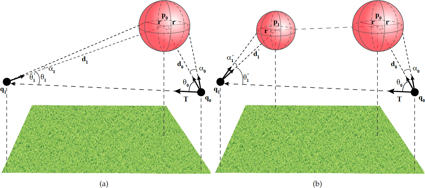
Determination of whether an object is moving or static. (a) Information about the UAS translation unit direction (T), the unit direction vectors (d₀ and d₁) connecting the UAS and the object and the expansion of its image between two camera frames. α₀ and α₁ represent the angular sizes of the images of the object in the two frames. A closed triangle is formed between the motion of the UAS (from position q₀ to position q₁) and the static object (at position p₀). (b) Primed symbols represent the angles and vectors, had the object moved between two frames.

At time t₁, when the aircraft has translated by the vector T, the object would be viewed in the direction θ₁ and would have an angular size α₁ – had it been stationary. However, if the object had moved during the period between t₁ and t₂ and now occupied a new position (p₁), it would be viewed from a different direction (θ₁') and would have a different angular size (α₁'). The viewing directions and angular sizes, as measured before and after the translation (i.e., at times t₀ and t₁), are used to infer the motion status of the object, as described below.

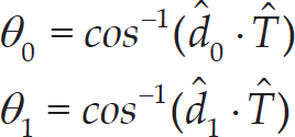
The vectors d₀ and d₁ are the directions from the quadrotor positions (q₀, q₁) to the object positions (p₀, p₁), respectively. These directions are determined by first computing the centroid of the image of the object, as discussed in Section 2.1, and then converting the pixel centroid to a 3D unit vector by using the camera model. The UAS translation vector and the object direction vectors are then used to compute the angles θ₀ and θ₁ using (3) below. Once these angles are computed, the change in the size of the object's image is used to determine the change in relative distance between the UAS and the object. Consider an object, in this case, a red ball, approaching the UAS. As the object approaches the vision system it will appear larger in the image, thus the angular size will increase (α₀ < α₁ in Fig. 3). The opposite would be true if the object were receding: the angular size will then decrease (α₀ > α₁ in Fig. 3). Therefore, the change in the size of the object in the image can be used to compute the change in distance (d₀ / d₁), as shown in (1). If the object were stationary, the change in distance (d₀ / d₁) would be equal to both the ratio of the tangent object's angular sizes from t₀ to t₁ (1), and the ratio of the sines of the angles θ₀ and θ₁ (2), as dictated by the geometry of a triangle:

\frac{‖ d_{0} ‖}{‖ d_{1} ‖} = \frac{s i n (θ_{1})}{s i n (θ_{0})}

(1)

\frac{‖ d_{0} ‖}{‖ d_{1} ‖} = \frac{t a n (α_{1})}{t a n (α_{0})}

(2)

where

\begin{array}{l} θ_{0} = c o s^{- 1} ({\hat{d}}_{0} \cdot \hat{T}) \\ θ_{1} = c o s^{- 1} ({\hat{d}}_{1} \cdot \hat{T}) \end{array}

(3)

and d₀ and T are unit vectors. As both (1) and (2) are equal to the ratio of the initial and final distances from a stationary object, the angles θ₀ and θ₁, and α₀ and α₁, would be related as shown in (4), below. However, this relationship only holds if the object is stationary. If the object is moving, there will be a disparity (δ)¹ between the expected change in distance (2) and the measured change in distance (1). This disparity value is calculated using (5), and is used to determine whether the object is moving or stationary.

\frac{s i n (θ_{1})}{s i n (θ_{0})} = \frac{t a n (α_{1})}{t a n (α_{0})}

(4)

δ = | | \frac{s i n (θ_{1})}{s i n (θ_{0})} - \frac{t a n (α_{1})}{t a n (α_{0})} | |

(5)

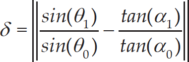
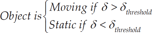
In theory, a stationary object would produce zero disparity (δ = 0), and a moving object would generate a non-zero disparity (δ ≠ 0). However, due to noise in the measurements of aircraft translation (egomotion), and in the measurements of the directions and sizes of the object in the images, even a stationary object will generate some disparity value. Therefore, a disparity threshold (δ_threshold) is used to classify the motion of the object as either moving or stationary, as shown in (6).

O b j e c t i s {\begin{array}{l} M o v i n g i f δ > δ_{t h r e s h o l d} \\ S t a t i c i f δ < δ_{t h r e s h o l d} \end{array}

(6)

A factor that influences the sensitivity of the detection of target motion is the angle between the directions of motion of both the target and the quadrotor. A smaller angle between these directions will produce a diminished disparity signal (for an extensive signal-to-noise analysis, see [36]). To improve the reliability of TCM, it is computed from two camera frames separated by an interval of 25 frames, as detailed below in Section 3.1. This frame interval increases the signal-to-noise ratios of the various angle measurements and provides more reliable results, provided that the computation of both optic flow and egomotion remain reliable over this larger inter-frame interval (which turns out to be the case in our experiments).

3 Optimizing TCM

To optimize the TCM algorithm, two control flight tests were conducted. In the first control flight, the object was stationary and in the second control flight, it was moving back and forth throughout the test – the motion was perpendicular to the quadrotor (T90), see Section 4. In Fig. 4 (a), the time course of the measured disparity is shown in red for the static object, and in green for the moving object. The green curve displays strong oscillations at twice the frequency of the oscillation of the object, because the disparity is either high or low according to whether the object is moving at a high speed (at the mid-point of its oscillatory trajectory) or at a speed close to zero (when its direction changes).

Figure 4.

Determination of separation between the disparity responses for a stationary object and a moving object for various frame intervals. (a) TCM disparity for a moving target (green) and a static target (red) to compute separation. μ_m (solid black) is the mean disparity value for the moving target, and σ_m (dashed black) is the corresponding standard deviation. μ_s (solid blue) is the mean disparity value for the static target, and σ_s (dashed blue) is the standard deviation. (b) Measured separations for frame step values ranging between [0, 40] frames. The dashed line is a third order polynomial fit with R² = 0.91.

The parameters that were optimized were the frame interval (the number of frames between comparisons) required to enhance the signal-to-noise ratio, and the threshold (δ_threshold) for classifying an object as either moving or stationary.

3.1 Optimizing the frame interval required to detect motion

To determine the best frame interval, a range of intervals ([0,40] frames) was trialled on the control data set. To obtain a metric of the effectiveness of each of the frame intervals, the separation between the moving target disparity and the static target disparity was calculated using (7) from the means and standard deviations of the disparity curves, as illustrated in Fig. 4 (a).

S e p a r a t i o n = (μ_{m} - σ_{m}) - (μ_{s} + σ_{s})

(7)

Fig. 4 (b) shows the calculated separation for various frame intervals. A negative separation means that classification between the moving and static targets will be less accurate because the disparity values for a moving target will overlap with the static disparity threshold, and vice versa. It is evident that the best separation (approximately 0.06) is obtained with a frame interval of 25 frames.

A frame interval of 25 frames is used throughout the testing of the TCM method as this interval produced the best separation between moving and static targets. Using this frame interval, we can now determine the optimal threshold for achieving maximum classification accuracy, as described below.

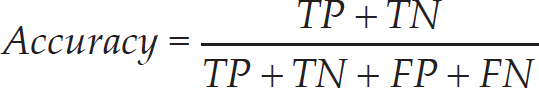
3.2 Computing threshold disparity for maximum classification accuracy

First, the accuracy of the method, as defined in (8), was used to provide a metric indicating the effectiveness of each threshold value. Here, TP is the number of True Positives, TN is the number of True Negatives, FP is the number of False Positives and FN is the number of False Negatives.

A c c u r a c y = \frac{T P + T N}{T P + T N + F P + F N}

(8)

Classification accuracy (8) was used to determine the optimum threshold disparity, δ_threshold, for reliable detection using the same control data.

As shown in Fig. 5, the disparity threshold varied between 0 and 1 to determine the value for the best classification accuracy. The optimum threshold was computed for various size images (shown in Table 1) to determine the effect of image resolution on both the threshold and the accuracy of the classifier.

Figure 5.

Classification accuracy (green) as a function of the disparity threshold for TCM (360×220 pixel image). The false positive rate (red) and true positive rate (blue) are also illustrated for different thresholds.

Figure 6.

Our UAS set-up (a), a custom-built quadrotor used for outdoor flight tests (b) and a unique panoramic vision system (c)

Table 1.

Optimal thresholds for the Triangle Closure Method (TCM) computed for various image resolutions (with the same field of view)

Image Resolution (pixels)	TCM
Image Resolution (pixels)	Max. Classifier Accuracy (%)	δ_threshold
360×220	95.44	0.084
540×330	96.63	0.078
720×440	95.13	0.087
900×550	91.14	0.081
1080×660	95.69	0.096

A threshold value of 0.09, corresponding to the average of the values shown in Table 1, was used for testing the TCM method.

4 Experimental Design

4.1 Flight platform

The UAS set-up used in our study, as shown in Fig. 6 (a), includes a laptop that is used merely to initiate the program on the quadrotor (no off-board processing is conducted on the laptop), a Differential GPS (DGPS) base station for ground truth and the quadrotor. The custom-built quadrotor (Fig. 6 (b)) comprises a MicroKopter flight controller. Data obtained by the onboard sensors and the vision system are processed using an Intel NUC, featuring an Intel i5 core 2.6GHz dual-core processor, 8GB of RAM and a 120GB SSD. The platform also carries a MicroStrain 3DM-GX3-25 Attitude and Heading Reference System (AHRS), a Ublox 3DR global positioning system (GPS), a Swift Navigation Piksi DGPS and a vision system, as illustrated in Fig. 6 (c). Note that the GPS and DGPS are only used for obtaining the ground truth, and are not used for navigation.

The vision system consists of two fisheye cameras (Point Grey Firefly MV cameras, Sunex DSL216 lenses). The cameras have a 25Hz frame rate. They are software synchronized and mounted back-to-back. Synchronized frames from the two cameras are stitched together using a camera calibration similar to that described in [41] to produce a panoramic image with a 360° by 150° field of view (360 by 220 pixel resolution).

4.2 Field testing

Nine outdoor tests were conducted, broken into three scenarios: a static object (TS), an object moving at 45° to the quadrotor's trajectory (T45) and an object moving perpendicular to the quadrotor's trajectory (T90), as illustrated in Fig. 7. The object, a 75cm diameter ball, was either static (TS) or moved back and forth over a distance of approximately 2m along the two different axes (T45 and T90), as shown in Fig. 7 (a). The oscillation frequency of the ball was approximately 0.35Hz throughout all the T45 and T90 tests, where the quadrotor underwent oscillatory motion at a rate of approximately 0.1Hz. The centre of the ball was positioned at a height of 1m above the ground. The quadrotor flew in an approximately straight 3m trajectory back and forth along a trajectory to the left of the ball, at a height of 2m (see Fig. 7 (a) and Fig. 7 (b)).

4.3 Ground truth

To provide a verification of the Triangle Closure Method, information from the GPS and DGPS was used to obtain the ground truth (GT) trajectories of both the quadrotor and the moving object. The GPS information was used to log the translation direction (T in Fig. 3) of the quadrotor, and the DGPS information provided the instantaneous distance between the UAS and the object (d₀ and d₁ in Fig. 3). The GPS does not deliver reliable ground truth data for the absolute position but provides more accurate velocity measurements. Thus, the GPS provides an accurate estimate of the direction of travel. These parameters provide all of the requirements to compute the true motion disparity of the object, as explained in Section 2.3.

5 Experimental Results for TCM

In this section, we present the results of various tests of the Triangle Closure Method (TCM), using a disparity threshold of 0.09, a frame interval of 25 frames and an image size of 360×220 pixels. The results provide a quantitative measure for our vision-based classification algorithm by comparing performance against ground truth (GT) data obtained from the GPS and DGPS measurements (see Section 4.2 for a full description of field testing and GT determination). Fig. 8 (a-c) show the mean and standard deviation of the disparity values for each set of the three TS, T45 and T90 experiments (for detailed statistics on each, see Table 2).

Figure 7.

Experimental design. (a) Schematic plan depicting the motion of the quadrotor and the object for the three scenarios: a static object (TS), an object moving at 45° to the quadrotor's trajectory (T45) and an object moving perpendicular to the UAV translation (T90). Experimental set-ups illustrating the motions of the UAV and the target for T90 (b) and T45 (c).

Figure 8.

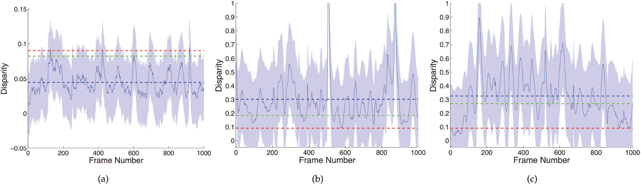
Mean and standard deviation disparities computed by TCM for the set of three tests within each scenario: (a) static object (TS), (b) object moving 45° to the translation direction (T45) and (c) object moving 90° to the translation direction (T90). The solid blue line and shading represent the mean and standard deviation of the three flight tests, respectively, while the blue dashed line is the overall mean of the disparity as computed by the vision-based TCM method. The green dashed line signifies the overall mean computed by the ground truth and the red line represents the disparity threshold.

Fig. 8 (a) displays the results for tests conducted with a stationary object. Here, the TCM data do not display the large periodic oscillations of Fig. 8 (b-c) because the target is not moving; however, there is still some oscillatory noise as the quadrotor moves back and forth. Fig. 8 (b-c) display the results of moving object tests (T45 and T90 conditions). In these cases, there are clear, periodic oscillations in the TCM.

It is possible to see that the majority of the data in the TCM curves and GT mean lines lie below the threshold of 0.09 with the static object (see Fig. 8 (a)), and above this threshold in the cases of the moving objects (see Fig. 8 (b) and Fig. 8 (c)). The larger oscillations and spikes in the T45 and T90 tests are due to the object and the UAS being moved back and forth in an oscillatory fashion, as described previously.

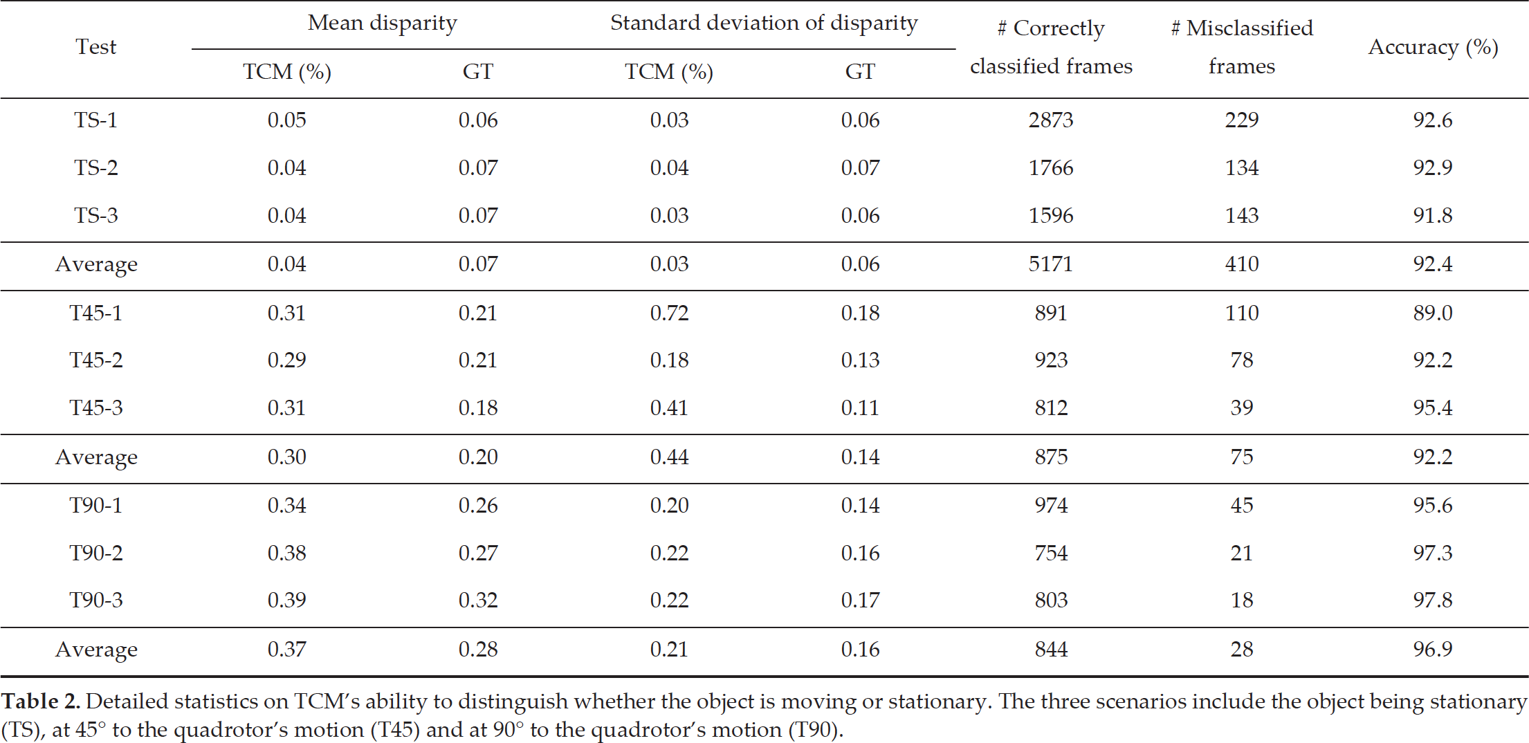
Table 2 provides an overview of the results for all the outdoor flight tests (TS, T45 and T90). Over the three static object tests (TS-1, TS-2 and TS-3), the mean disparity using the vision algorithm was found to be 0.04, with a standard deviation of 0.03. A mean of 0.07 and a standard deviation of 0.06 were calculated for the ground truth disparity. The average accuracy over the three static (TS) tests was determined to be 92.4% – where the classification accuracy was calculated according to (8).

The results for object motion at 45° to the UAS translation (T45) produced mean disparities of 0.30 and 0.20, respecttively, for the TCM results and the ground truth data, with corresponding standard deviations of 0.44 and 0.14. As in the static object experiments, the mean detection accuracy for the T45 tests was 92.2%.

Finally, the mean disparity for the T90 tests using the vision algorithm was found to be 0.37 with a standard deviation of 0.21, and a mean disparity of 0.28 and a standard deviation of 0.16 were calculated for the ground truth disparity. The average accuracy for the T90 experiments was 96.9%.

6 Comparison of the Triangle Closure Method, Background Subtraction Method and Epipolar Constraint Method

Two control flight tests were used to compare the performance of the Triangle Closure Method, Epipolar Constraint Method and the Background Subtraction Method. The object was stationary in the first control flight, and was moving back and forth throughout the test in the second. As in Section 5, in all of these tests, the centre of the object was raised 1m above the ground.

Table 2.
Detailed statistics on TCM's ability to distinguish whether the object is moving or stationary. The three scenarios include the object being stationary (TS), at 45° to the quadrotor's motion (T45) and at 90° to the quadrotor's motion (T90).

Test Mean disparity Standard deviation of disparity # Correctly classified frames # Misclassified frames Accuracy (%)

TCM (%) GT TCM (%) GT

TS-1 0.05 0.06 0.03 0.06 2873 229 92.6

TS-2 0.04 0.07 0.04 0.07 1766 134 92.9

TS-3 0.04 0.07 0.03 0.06 1596 143 91.8

Average 0.04 0.07 0.03 0.06 5171 410 92.4

T45-1 0.31 0.21 0.72 0.18 891 110 89.0

T45-2 0.29 0.21 0.18 0.13 923 78 92.2

T45-3 0.31 0.18 0.41 0.11 812 39 95.4

Average 0.30 0.20 0.44 0.14 875 75 92.2

T90-1 0.34 0.26 0.20 0.14 974 45 95.6

T90-2 0.38 0.27 0.22 0.16 754 21 97.3

T90-3 0.39 0.32 0.22 0.17 803 18 97.8

Average 0.37 0.28 0.21 0.16 844 28 96.9

Test	Mean disparity	Standard deviation of disparity	# Correctly classified frames	# Misclassified frames	Accuracy (%)
TS-1	0.05	0.06	0.03	0.06	2873	229	92.6
TS-2	0.04	0.07	0.04	0.07	1766	134	92.9
TS-3	0.04	0.07	0.03	0.06	1596	143	91.8

Average	0.04	0.07	0.03	0.06	5171	410	92.4

T45-1	0.31	0.21	0.72	0.18	891	110	89.0
T45-2	0.29	0.21	0.18	0.13	923	78	92.2
T45-3	0.31	0.18	0.41	0.11	812	39	95.4

Average	0.30	0.20	0.44	0.14	875	75	92.2

T90-1	0.34	0.26	0.20	0.14	974	45	95.6
T90-2	0.38	0.27	0.22	0.16	754	21	97.3
T90-3	0.39	0.32	0.22	0.17	803	18	97.8

Average	0.37	0.28	0.21	0.16	844	28	96.9

6.1 Background Subtraction Method (BSM)

The performance of TCM was compared with that of the Background Subtraction Method (BSM), which is a traditional technique that is widely used for the detection of a moving object. Background subtraction has been implemented for detecting moving objects from a stationary vision system, and occasionally from a moving vision system.

This section describes the Background Subtraction Method we used to detect moving objects from a UAS. To perform background subtraction using a moving platform, the rotation and translation of the UAS must be accounted for. In this paper, optic flow is used to compute the aircraft's egomotion, and the motion of an object is detected by sensing the motion parallax between the object and the background. The translation and rotation of the aircraft are computed using the same optic flow algorithm as described in Section 2 [38, 39]. Using the computed egomotion, the current frame is de-rotated and each pixel on the ground plane is de-translated into the previous frame. The same 25-frame interval is used as in TCM. Once the egomotion is accounted for in the current frame, the absolute frame difference is computed between the current and previous frames. This operation highlights the image of any object that moves relative to the image of the ground plane. The moving object is then detected by applying a pixel-wise threshold to the absolute difference image. This binary image is then used to detect moving objects by summing the number of pixels equal to 1, and applying a detection threshold.

For BSM, the threshold for detecting whether an object is moving or stationary is related to the number of suprathreshold pixels detected, as shown in Fig. 13 (c) and Fig. 14 (c). The range of thresholds examined to optimize the BSM classifier was [0,1000]. As with TCM, the optimum thresholds for the BSM were computed for various image resolutions (shown in Table 3).

6.2 Epipolar Constraint Method (ECM)

The Epipolar Constraint Method (ECM) can be used to determine whether an object is moving or stationary due to the geometric relationship between two image frames [42, 23]. It is shown in Fig. 9 (a) that the two UAS locations q₀ and q₁ (i.e., the two camera viewpoints in 3D space) and the world point P defines a plane – this plane is also known as the epipolar plane. Now let ⁰p and ¹p define the two points represented by the projection of the world point P onto the two image frames at the locations q₀ and q₁, respectively, which are known as conjugate points, as discussed in [42]. In our case, the image locations ⁰p and ¹p are determined by the colour-based method discussed in Section 2.2. These conjugate points define the directions of the target when it is viewed from locations q₀ and q₁, respectively. These directions are denoted by the vectors o₀ and o₁. The vectors t and o₀ define the epipolar constraint plane, whose normal is denoted by the vector n₀. We can determine whether the object remains in the epipolar plane after the quadrotor has moved to q₁ by computing the normal to t and o₁, dented by n₁ and examining whether n₁ is parallel to n₀. If n₁ is parallel to n₀, the object lies in the epipolar plane and is inferred not to have moved, as illustrated in Fig. 9 (a). If n₁ is not parallel to n₀, the object no longer lies in the epipolar plane and is inferred to have moved, as illustrated in Fig. 9 (b).

In order to determine whether the two direction vectors o₀ and o₁ conform to the epipolar plane constraint, the normal vectors n₀ and n₁ are computed by the cross products n₀ =t x o₀ and n₁ = t x o₁. To determine whether the direction vectors o₀ and o₁ satisfy the epipolar plane constraint, the angle (Ω) between n₀ and n₁ is computed, where:

Figure 9.

Determination of whether an object is stationary (a) or moving (b) using ECM. Information about the UAS translation unit direction (t) and the unit direction vectors (o₀ and o₁) connecting the UAS and the object are required between two camera frames for ECM.

Table 3.

Performance of TCM compared to those of ECM and BSM for various image resolutions

Image Res. (pixel)	TCM			ECM			BSM
Image Res. (pixel)	ROC Area (%)	Max. accuracy (%)	Disparity Threshold	ROC Area (%)	Max. accuracy (%)	Disparity Threshold (degrees) ROC Area (%)	Max. accuracy (%)	Threshold (pixels)
360×220	96.46	95.44	0.084	96.09	88.81	0.072	61.53	57.78	7
540×330	96.62	96.63	0.078	95.53	87.61	0.052	78.55	73.03	56
720×440	96.47	95.13	0.087	95.38	87.11	0.056	82.45	77.03	145
900×550	94.83	91.14	0.081	95.50	87.36	0.056	83.01	77.28	317
1080×660	95.69	94.32	0.096	95.40	86.91	0.049	81.98	77.22	495

Objectis {\begin{array}{l} M o v i n g i f Ω > Ω_{t h r e s h o l d} \\ S t a t i c i f Ω < Ω_{t h r e s h o l d} \end{array}

(9)

Here, the object is deemed to be moving when the angle between the normal vectors, Ω, is greater than the threshold (Ω_threshold). Fig. 9 (a) illustrates a static object whereby the two direction vectors satisfy the epipolar plane constraint (i.e., n₀ = n₁) and Fig. 9 (b) demonstrates a moving object that breaks the geometric constraints of the epipolar plane (i.e., n₀ ≠ n₁).

The threshold for detecting whether an object is moving or stationary for ECM is based on the angular disparity between the two normal vectors n₀ and n₁. The range of thresholds explored in order to determine the optimal threshold for maximum accuracy was [0,1]. As with TCM and BSM, the optimum thresholds for the ECM were computed for various image resolutions (shown in Table 3).

6.3 Performance evaluation

By knowing that in one test the object was always static and in the other it was constantly moving, the true positives (TP) (where a true positive is a moving object that is detected to be in motion) and true negatives (TN), and the false positives (FP) and false negatives (FN), were computed for various threshold levels at different image resolutions. The reliability of detection was evaluated by calculating a Receiver Operating Characteristic (ROC) plot, which includes TP, TN, FP and FN values.

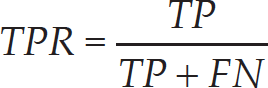
Once the statistics were computed for TCM, ECM and BSM with varying thresholds, a ROC curve was plotted for each method. The ROC curve is a plot of the False Positive Rate (FPR), calculated by (10), compared to the True Positive Rate (TPR), calculated by (11). The area under the ROC curve quantifies the ability of the method to distinguish reliably between a moving and a static target – an area of 1 represents a perfect classifier. To compare the performance of the different techniques discussed in this paper, the maximum accuracy, ROC area and optimal thresholds are determined for various image sizes, as shown in Table 3.

T P R = \frac{T P}{T P + F N}

(10)

F P R = \frac{F P}{F P + T N}

(11)

Each method was evaluated for various image resolutions, to determine the optimum threshold and the effects on classification accuracy. It is observed that the Background Subtraction Method increases in accuracy from 57.87% for a 360×220 pixel image to a maximum accuracy of 77.28% for a 900×550 pixel image, and then marginally reduces in accuracy for the largest image size. On the other hand, the accuracy rates of TCM and ECM remain approximately constant. ECM has an accuracy of approximately 87% compared to TCM's maximum accuracy, which is above 90% across the different image resolutions. It is also interesting to note that the optimum threshold for the Background Subtraction Method increases with image resolution, whereas the optimum thresholds for the Triangle Closure Method and Epipolar Constraint Method are invariant. Thus, TCM and ECM provide more reliable approaches that can be used with image resolutions to suit a range of applications, without requiring a change or re-exploration of the optimum threshold parameters.

Although the performance of the Background Subtraction Method improves with higher image resolutions, it never attains the accuracy of either TCM and ECM even at the highest image resolution. Furthermore, the Background Subtraction Method works best with high image resolutions, which is often not feasible in real-time applications.

The ROC plot in Fig. 10 compares the performance of TCM (green curve), ECM (blue curve) and BSM (black curve). The optimal image size of 900×550 pixels is used for the Background Subtraction Method, compared to the 360×220 pixel image size for TCM and ECM. The reason for using the smallest image size for TCM (although it is slightly less accurate) is the computational cost, as discussed in the next section. It is clear that TCM demonstrates higher reliability than either ECM or BSM, despite the greater image resolution used for the BSM.

Figure 10.

ROC plot comparing the performance of the Triangle Closure Method (TCM) (green) (320×220 pixel resolution) with that of the Epipolar Constraint Method (ECM) (blue) (320×220 pixel resolution) and the Background Subtraction Method (BSM) (black) (900×550 pixel resolution)

6.4 Computation time

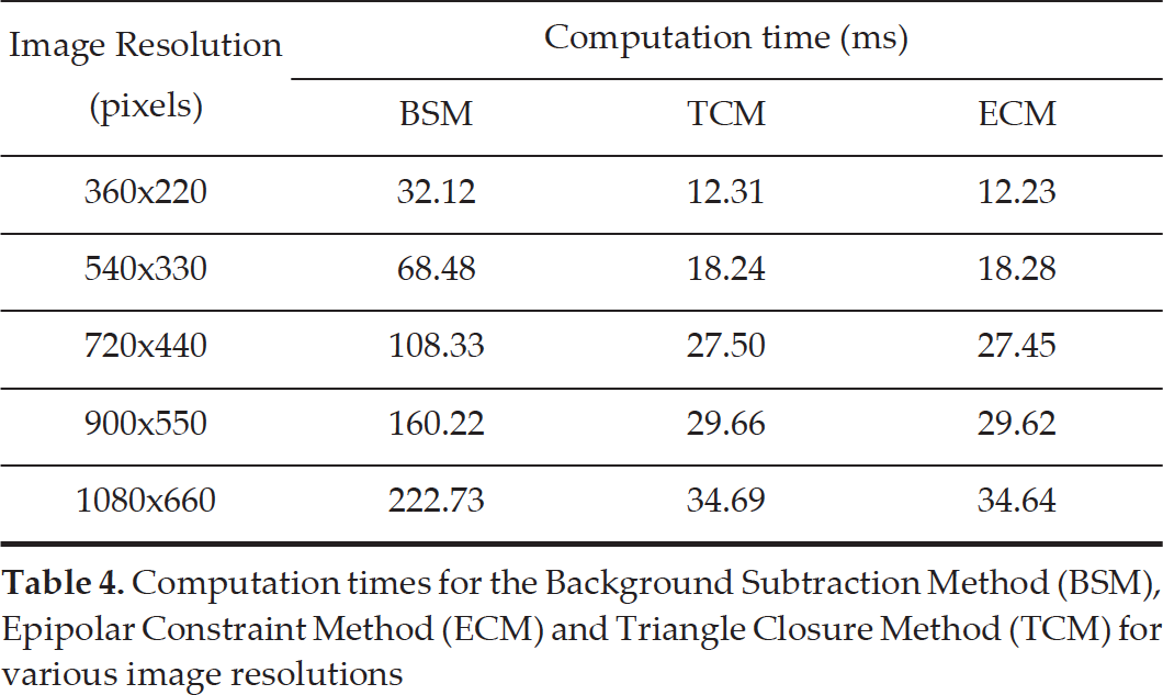
The time that it takes to detect an object and classify its motion status could make the critical difference between avoiding an object and colliding with it. To compare the timings of the three methods described in this paper, all techniques were tested under the same conditions, using the same image resolutions. Table 4 summarizes the computation time for each method for various image resolutions. It is evident that the Triangle Closure Method is computationally faster than the Background Subtraction Method. For the 360×220 pixel resolution, which was used on the platform, background subtraction took approximately 32ms per frame, compared to our Triangle Closure Method, which requires only about 12ms. In terms of computation time, the performance of ECM is very similar to that of TCM, as both utilize the same colour-detection algorithm – both approaches are significantly faster than the BSM.

Table 4.
Computation times for the Background Subtraction Method (BSM), Epipolar Constraint Method (ECM) and Triangle Closure Method (TCM) for various image resolutions

Image Resolution (pixels) Computation time (ms)

BSM TCM ECM

360×220 32.12 12.31 12.23

540×330 68.48 18.24 18.28

720×440 108.33 27.50 27.45

900×550 160.22 29.66 29.62

1080×660 222.73 34.69 34.64

Image Resolution (pixels)	Computation time (ms)
360×220	32.12	12.31	12.23
540×330	68.48	18.24	18.28
720×440	108.33	27.50	27.45
900×550	160.22	29.66	29.62
1080×660	222.73	34.69	34.64

For a UAS to fly autonomously it needs to be able to process all data in real time – in this paper, real time is considered to be 40ms, corresponding to a standard video frame rate of 25Hz or faster. All timings were measured on the flight computer (see Section 4.1 for additional information). The fastest processing time for the BSM is approximately 32.12ms. Even though the processing time for the BSM is below 40ms, when other processes such as image preprocessing, stereo height computation and optic flow – all of which run in under 13ms on a 320×220 pixel image – are factored into the computation time, the total processing time for BSM increases to over 45ms. With the TCM, on the other hand, all processing can be completed in less than 25ms, which is well below the 40ms requirement. Note that no additional optimizations have been implemented into either method. Admittedly, it is possible to optimize the BSM method by using a graphical processing unit (GPU).

6.5 Limitations of the methods

6.5.1 TCM

One limitation that would compromise the ability of TCM to detect a moving object is when the object moves along a head-on collision trajectory. However, the TCM already employs looming cues, which could be used on their own to determine the time to collision and to initiate an evasive manoeuvre. This idea of time to contact (TTC) is well studied: for example, plummeting gannets use TTC to retract their wings before diving into water [43]. Secondly, an object that moves along a trajectory parallel to that of the UAS will generate the same disparity (zero) as a stationary object at a greater distance, as is illustrated in Fig. 11 (a), and will therefore be deemed to be stationary: d₁ / d₂ = D₁ / D₂. On the other hand, an object that moves in a direction different to that of the quadrotor (e.g., Fig. 11 (b)) will always generate a non-zero disparity (d₁ / d₂ ≠ D₁ / D₂) and will therefore always be accurately classified as moving. In the special case of parallel motion, the object moves in such a way as to conceal its motion (‘motion camouflage’, as described by [44]), and is therefore undetectable by any monocular vision-based algorithm, including ours. However, such an object is not a potential threat, as it would always be at a safe distance away from the UAS.

Figure 11.

Object moving parallel (a) and non-parallel (b) to the aircraft

In this work, we have assumed that the object is spherical. Therefore, the shape of the object's image is always a circle, regardless of the viewing direction. This simplifies the task of computing changes in the distance between the object and the UAS – it is only necessary to measure the change in the size of the object's image, in terms of pixel coverage. The situation would be more complex, however, if the object's shape is very unlike that of a sphere, because the shape of the image would then vary depending upon the viewing direction, and the image size would not be directly related to the object's distance. This problem could be solved by tracking the distance between two distinct features on the object, or by evaluating the change in image size along an axis perpendicular to the UAS's translation direction.

6.5.2 ECM

Although ECM does not require the spherical assumption as in TCM, the ECM has a crucial shortcoming. Consider, again, the two direction unit vectors o₀ and o₁, as illustrated in Fig. 9 (a). An object can fool the ECM if it were to move in such a way as to ensure that the direction vector o₁ crossed with the translation vector t, producing the same normal vector n₁ as when it had while being static. That is, the target is deemed to be static when it is, in fact, moving. One such example is highlighted in the data set used to compare the three methods, where the object and quadrotor move in such a way that the direction of the target in the visual field of the quadrotor's vision system (the position in the image frame captured by the vision system) remained constant, as is demonstrated by the video sequence in Fig. 12 (b) and is further explained by the schematic in Fig. 12 (d). The object can only be detected if the epipolar constraint is violated as shown in Fig. 12 (a) and Fig. 12 (c). On the other hand, TCM will correctly classify the object as moving because it additionally monitors the image size of the target.

6.5.3 BSM

Fig. 13 and Fig. 14 illustrate the performance of the background subtraction algorithm. The algorithm reports the object to be moving in the examples of Fig. 13 as well as Fig. 14; however, motion was only present in the example of Fig. 13. Thus, the Background Subtraction Method erroneously reports the object as moving even in Fig. 14, when in reality it is static – the opposite problem to that of the ECM. This is because the stationary object produces motion contrast against the background when it is raised above the background.

7 Discussion

TCM was able to correctly classify whether the object was stationary or moving in three test scenarios: a static object (TS), an object moving at 45° to the quadrotor's trajectory (T45) and an object moving perpendicular to the quadrotor's trajectory (T90). In all of these cases, the quadrotor was translating back and forth (see Section 4.2 for further details). It is possible to detect whether an object is moving or static with a variety of angles between the quadrotor and target translation directions; however, in this paper, only a subset of directions were used to demonstrate the effectiveness of TCM.

To evaluate the accuracy of TCM, the algorithm was compared against ground truth data from the GPS, which provided information on the translation of the aircraft, and the DGPS provided information on the relative distance and the direction to the object. The update rates for the GPS and DGPS are 5Hz; thus, there are discrepancies between the ground truth and the TCM algorithm, which runs in real time at 25Hz. Even with these differences in sampling rates, the signals as computed by TCM correlated with the ground truth data.

The Triangle Closure Method is also shown to have overcome some of the limitations of both the Background Subtraction Method and the Epipolar Constraint Method. One of the major limitations that is solved by TCM and not by BSM is the occurrence of false detections due to the motion parallax that is generated when a stationary object is not a part of the dominant plane – here, the dominant plane is used to compute motion contrast between frames. Thus, an object such as a lamp post or an elevated ball (as in this experiment) is misclassified as a moving object when it is in fact static, as illustrated in Fig. 14 (c). There have been studies to remove the effect of parallax, as in [45]; however, this requires an additional step that could potentially be computationally expensive. Our method, as explained in Section 2.3, avoids this limitation and can even be utilized as an additional step for obtaining greater reliability when motion-contrast methods are used. In addition, our method does not require the object to be viewed against a planar background. The background can have any structure, or even be absent (as when an object is perceived against a clear sky).

Figure 12.

Using the ECM to demonstrate its ability to determine whether an object is moving or stationary within the T90-1 experimental data set. Video sequences are separated by five frames, from top to bottom. (a) shows that the target is determined to be moving as it violates the epipolar constraint as illustrated by (c). (b) provides an example in which the ECM method is fooled by the motion of the target and the UAS, as is illustrated by (d).

Figure 13.

Example of a test of the BSM on a moving platform, for an object that is static and raised 1m above the ground. (a) illustrates the stitched images from the on-board camera system. (b) is the egomotion-compensated subtraction of two frames that are 25 frames apart. (c) is an inset for a section of (b) that thresholds for moving objects based on pixel intensity differences in the resulting difference image.

Figure 14.

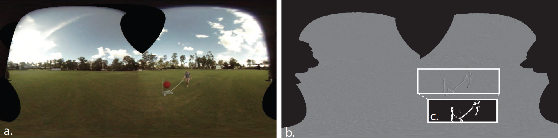
Example of a test of the BSM on a moving platform, for an object that is moving and raised 1m above the ground. (a) illustrates the stitched images from the on-board camera system. (b) is the egomotion-compensated subtraction of two frames that are 25 frames apart. (c) is an inset for a section of (b) that thresholds for moving objects based on pixel intensity differences in the resulting difference image.

TCM also provides a different method for classifying the motion of an object compared to the well-known Epipolar Constraint Techniques. TCM does not use or require stereo. Rather, it compares the ratio of the predicted distances to the target with the measured expansion ratio of the object images, as discussed in Section 2.3. The main problem overcome by TCM when compared to the Epipolar Constraint Method is the issue that arises when the ECM determines an object to be static when, in fact, it is moving along the epipolar constraint – these false negatives are shown by the reduced area of the epipolar constraint's ROC compared to TCM, which is explained by the increased FNs in (10). In this instance, TCM can still correctly determine that the target is moving as it utilizes the expansion of the object in the image.

The performances of TCM, ECM and BSM are evaluated and compared in Section 6 by comparing the thresholds, ROC curves, accuracies and computation times. The area under the ROC plot gives an indication of the overall performance of the system, where an area of 1 (or 100%) represents a perfect classifier. Using the optimal image size (900×550), a ROC area of 83% was computed for the Background Subtraction Method, with a maximum accuracy of 77%. The Epipolar Constraint Method scored an area of 83% on the ROC curve with an 88% accuracy. On the other hand, our TCM method achieves a ROC area of 96% and a maximum accuracy of 95%. It is clear that both the ECM and TCM outperform the BSM, even when computed using a smaller image – this is also verified by [23], where in that study the epipolar technique outperformed homography background subtraction, rank constraint and fundamental matrix methods. By utilizing smaller images and delivering better accuracy, the TCM method provides improved results with a reduction in computation time. The classification accuracy was also used to determine the optimal threshold for each method. It is clear from these tests that our Triangle Closure Method is preferable to the background subtraction technique, because TCM can use a singe threshold that is independent of image size.

Our method was able to correctly classify the motion of the test object, as verified by ground truth measurements for a number of scenarios in each of the experiments. The TS, T45 and T90 scenarios demonstrated accuracies of 92.4, 92.2% and 96.9%, respectively. The slightly smaller accuracy with the T45 test as compared to that of the T90 is not surprising, given the smaller angle between the axes of motion for the quadrotor and the moving object in this case. A smaller θ₀ or θ₁ will produce a smaller disparity, and if θ₀ = 0 in Section 2.2, the disparity is undefined. For a full noise and sensitivity analysis, refer to [36]. Although the Triangle Closure Method has its limitations, it does addresses a number of current issues in the literature for determining whether an object is moving or static, as discussed in the Section 1.

7.1 Applications

As we are on the cusp of UAS integration into regulated airspace, it is paramount that safety regulations reflect the need for aircraft with situational awareness, in order to minimize the risk of potentially fatal accidents. This is especially critical at the moment, given the rapidly increasing number of UAS and remotely piloted hobby aircraft flying at low altitudes.

The work presented here focuses on this problem by providing a moving platform with the capacity to classify objects as either moving or stationary at low altitudes. Through use of vision-based techniques we can significantly improve our understanding of the surrounding environment, which in turn allows for better control decisions, such as timely and effective evasive manoeuvres, therefore improving aviation safety. Our TCM method can be implemented on various robots (ground and air) and, although this paper uses a vision-based approach, other sensors such as laser rangefinders and the GPS could be utilized to determine the parameters in Fig. 3.

8 Conclusions

This paper describes a technique, the Triangle Closure Method (TCM), to determine whether an object in proximity to a moving vision system is stationary or moving. We show that TCM, which utilizes the aircraft's translation inferred from the optic flow and the change in size of the object's image, provides an accurate and robust classification of an object's motion status. In field tests, TCM performed better than a traditional background subtraction algorithm and the Epipolar Constraint Method. In summary, the key findings of this study are:

Techniques that rely simply on motion contrast can misclassify stationary objects as being in motion if they are at a different distance to the background (or on the dominant plane).

The epipolar constraint by itself can be fooled when an object moves along the epipolar constraint.

Combining the UAS's egomotion estimate with the object's expansion, as is done in TCM, can overcome some of the limitations of BSM and ECM.

TCM correctly distinguishes between an object that is moving compared to one that is stationary, in a number of scenarios tested onboard a UAS in outdoor conditions.

The major reason for the better performance of TCM is that it overcomes the limitations of other methods, such as various types of background subtraction that are subject to false detections (false positives) of movement introduced by the presence of motion contrast or Epipolar Constraint Methods that can produce false negatives when the object is moving on the constraint plane. Finally, the TCM is a versatile approach for determining whether objects are moving or stationary, which can be implemented on terrestrial and aerial vehicles to facilitate improved control decisions such as timely evasive manoeuvres, thus improving overall transport safety.

Footnotes

Acknowledgements

This article is a revised and expanded version of a paper entitled “TCM: A Fast Technique to Determine if an Object is Moving or Stationary from a UAV”, presented at the Australasian Conference on Robotics and Automation (ACRA) 2015 in Canberra, Australia.

The research described here was supported partly by the Boeing Defence Australia Grant SMP-BRT-11-044, ARC Linkage Grant LP130100483, ARC Discovery Grant DP140100896, a Queensland Premier's Fellowship and an ARC Distinguished Outstanding Researcher Award (DP140100914). We thank Dean Soccol for his assistance with the mechanical aspects of this work.

1

δ is a dimensionless quantity, as it is the difference between two ratios.

References

Lai

John

Ford

Jason J

Mejias

Luis

O'Shea

Peter

. Characterization of sky-region morphological-temporal airborne collision detection. Journal of Field Robotics, 30(2):171–193, 2013.

Nussberger

Andreas

Grabner

Helmut

Van Gool

Luc

. Aerial object tracking from an airborne platform. In Unmanned Aircraft Systems (ICUAS), 2014 International Conference on, pages 1284–1293. IEEE, 2014.

Clothier

Reece

Frousheger

Dennis

Wilson

Michael

Grant

. The smart skies project: Enabling technologies for future airspace environments. In 28th Congress of the International Council of the Aeronautical Sciences. ICAS, 2012.

Wilson

Michael

. Ground-based sense and avoid support for unmanned aircraft systems. Congress of the International Council of the Aeronautical Sciences (ICAS), 2012.

Korn

Bernd

Edinger

Christiane

. UAS in civil airspace: Demonstrating “sense and avoid™ capabilities in flight trials. In Digital Avionics Systems Conference, 2008. DASC 2008. IEEE/AIAA 27th, pages 1–7. IEEE, 2008.

Viquerat

Andrew

Blackhall

Lachlan

Reid

Alistair

Sukkarieh

Salah

Brooker

Graham

. Reactive collision avoidance for unmanned aerial vehicles using doppler radar. In Field and Service Robotics, pages 245–254. Springer, 2008.

Green

William E

Paul Y

Barrows

Geoffrey

. Flying insect inspired vision for autonomous aerial robot maneuvers in near-earth environments. In Robotics and Automation, 2004. Proceedings. ICRA'04. 2004 IEEE International Conference on, volume 3, pages 2347–2352. IEEE, 2004.

Zufferey

Jean-Christophe

Floreano

Dario

. Fly-inspired visual steering of an ultralight indoor aircraft. Robotics, IEEE Transactions on, 22(1):137–146, 2006.

Denuelle

Aymeric

Thurrowgood

Saul

Strydom

Reuben

Kendoul

Farid

Srinivasan

Mandyam V

. Biologically-inspired visual stabilization of a rotorcraft UAV in unknown outdoor environments. In Unmanned Aircraft Systems (ICUAS), 2015 International Conference on, pages 1084–1093. IEEE, 2015.

10.

Srinivasan

Mandyam V

. Visual control of navigation in insects and its relevance for robotics. Current opinion in neurobiology, 21(4):535–543, 2011.

11.

Zabala

Francisco

Polidoro

Peter

Robie

Alice

Branson

Kristin

Perona

Pietro

Dickinson

Michael H

. A simple strategy for detecting moving objects during locomotion revealed by animal-robot interactions. Current Biology, 22(14):1344–1350, 2012.

12.

Spagnolo

Paolo

Leo

Distante

. Moving object segmentation by background subtraction and temporal analysis. Image and Vision Computing, 24(5):411–423, 2006.

13.

Sobral

Andrews

Vacavant

Antoine

. A comprehensive review of background subtraction algorithms evaluated with synthetic and real videos. Computer Vision and Image Understanding, 122:4–21, 2014.

14.

Benezeth

Yannick

Jodoin

P-M

Emile

Bruno

Laurent

Hélene

Rosenberger

Christophe

. Review and evaluation of commonly-implemented background subtraction algorithms. In Pattern Recognition, 2008. ICPR 2008. 19th International Conference on, pages 1–4. IEEE, 2008.

15.

Denman

Simon

Fookes

Clinton

Sridharan

Sridha

. Improved simultaneous computation of motion detection and optical flow for object tracking. In Digital Image Computing: Techniques and Applications, 2009. DICTA'09., pages 175–182. IEEE, 2009.

16.

Butler

Darren

Sridharan

Sridha

Bove

V Michael

Jr . Real-time adaptive background segmentation. In Acoustics, Speech, and Signal Processing, 2003. Proceedings.(ICASSP'03). 2003 IEEE International Conference on, volume 3, pages 349–52. IEEE, 2003.

17.

Lucas

Bruce D

Kanade

Takeo

. An iterative image registration technique with an application to stereo vision. In IJCAI, volume 81, pages 674–679, 1981.

18.

Horn

Berthold K

Schunck

Brian G

. Determining optical flow. In 1981 Technical symposium east, pages 319–331. International Society for Optics and Photonics, 1981.

19.

Choi

Jay Hyuk

Lee

Dongjin

Bang

Hyochoong

. Tracking an unknown moving target from uav: Extracting and localizing an moving target with vision sensor based on optical flow. In Automation, Robotics and Applications (ICARA), 2011 5th International Conference on, pages 384–389. IEEE, 2011.

20.

Tian

Ying-Li

Hampapur

Arun

. Robust salient motion detection with complex background for real-time video surveillance. In Application of Computer Vision, 2005. WACV/MOTIONS'05 Volume 1. Seventh IEEE Workshops on, volume 2, pages 30–35. IEEE, 2005.

21.

Wixson

. Detecting salient motion by accumulating directionally-consistent flow. Pattern Analysis and Machine Intelligence, IEEE Transactions on, 22(8): 774–780, 2000.

22.

Strydom

Reuben

Thurrowgood

Saul

Srinivasan

Mandyam V

. Airborne vision system for the detection of moving objects. In Australasian Conference on Robotics and Automation (ACRA), pages 1–7. Australian Robotics and Automation Association, 2013.

23.

Dey

Soumyabrata

Reilly

Vladimir

Saleemi

Imran

Shah

Mubarak

. Detection of independently moving objects in non-planar scenes via multi-frame monocular epipolar constraint, pages 860–873. Springer, 2012.

24.

In Kim

Choi

Hong Seok

Kwang Moo

Choi

Jin Young

Kong

Seong G

. Intelligent visual surveillance—a survey. International Journal of Control, Automation and Systems, 8(5):926–939, 2010.

25.

Pinto

Andry Maykol

Costa

Paulo Gomes

Moreira

António Paulo

. Introduction to visual motion analysis for mobile robots. In CONTROLO'2014–Proceedings of the 11th Portuguese Conference on Automatic Control, pages 545–554. Springer, 2015.

26.

Sun

Zehang

Bebis

George

Miller

Ronald

. On-road vehicle detection: A review. Pattern Analysis and Machine Intelligence, IEEE Transactions on, 28(5): 694–711, 2006.

27.

Yuan

Ding

Yalong

. Moving object detection under moving camera by using normal flows. Robotics and Biomimetics (ROBIO), 2014 IEEE International Conference on, 2014.

28.

Thakoor

Ninad

Gao

Jean

Chen

Huamei

. Automatic object detection in video sequences with camera in motion. In Proceedings of Advanced Concepts for Intelligent Vision Systems. Citeseer, 2004.

29.

Sundaram

Narayanan

Brox

Thomas

Keutzer

Kurt

. Dense point trajectories by GPU-accelerated large displacement optical flow, pages 438–451. Springer, 2010.

30.

Bouwmans

Thierry

. Traditional and recent approaches in background modeling for foreground detection: An overview. Computer Science Review, 11:31–66

31.

Singh

Deepak

Kumar

Praveen

. A comparative study on various background subtraction mechanisms for motion detection. International Journal of Advanced Electronics and Communication Systems, 3(5), 2014.

32.

Hayman

Eric

Eklundh

Jan-Olof

. Statistical background subtraction for a mobile observer. In Computer Vision, 2003. Proceedings. Ninth IEEE International Conference on, pages 67–74. IEEE, 2003.

33.

Sugaya

Yasuyuki

Kanatani

Kenichi

. Extracting moving objects from a moving camera video sequence. In Proceedings of the 10th Symposium on Sensing via Imaging Information, pages 279–284, 2004.

34.

Taneja

Aparna

Ballan

Luca

Pollefeys

Marc

. Modeling dynamic scenes recorded with freely moving cameras, pages 613–626. Springer, 2011.

35.

Elqursh

Ali

Elgammal

Ahmed

. Online moving camera background subtraction, pages 228–241. Springer, 2012.

36.

Strydom

Reuben

Thurrowgood

Saul

Srinivasan

Mandyam V

. TCM: A fast technique to determine if an object is moving or stationary from a UAV. In Australasian Conference on Robotics and Automation (ACRA). Australian Robotics and Automation Association, 2015.

37.

Strydom

Reuben

Thurrowgood

Saul

Denuelle

Aymeric

Srinivasan

Mandyam V

. UAV Guidance: A Stereo-Based Technique for Interception of Stationary or Moving Targets, In Towards Autonomous Robotic Systems (TAROS) pages 258–269. Springer, 2015.

38.

Thurrowgood

Saul

Moore

Richard JD

Soccol

Dean

Knight

Michael

Srinivasan

Mandyam V

. A biologically inspired, vision-based guidance system for automatic landing of a fixed-wing aircraft. Journal of Field Robotics, 31(4):699–727, 2014.

39.

Strydom

Reuben

Thurrowgood

Saul

Srinivasan

Mandyam V

. Visual odometry: Autonomous uav navigation using optic flow and stereo. In Australasian Conference on Robotics and Automation (ACRA), pages 1–10. Australian Robotics and Automation Association, 2014.

40.

Jouir

Tasarinan

Strydom

Reuben

Srinivasan

Mandyam V

. A 3D sky compass to achieve robust estimation of UAV attitude. In Australasian Conference on Robotics and Automation (ACRA). Australian Robotics and Automation Association, 2015.

41.

Kannala

Juho

Brandt

Sami S

. A generic camera model and calibration method for conventional, wide-angle, and fish-eye lenses. Pattern Analysis and Machine Intelligence, IEEE Transactions on, 28(8): 1335–1340, 2006.

42.

Corke

Peter

. Robotics, vision and control: Fundamental algorithms in MATLAB, volume 73. Springer, 2011.

43.

Lee

Davis N

Reddish

Paul E

. Plummeting gannets: A paradigm of ecological optics. Nature, 1981.

44.

Srinivasan

Mandyam V

Davey

Matthew

. Strategies for active camouflage of motion. Proceedings of the Royal Society of London. Series B: Biological Sciences, 259(1354):19–25, 1995.

45.

Kang

Jinman

Cohen

Isaac

Medioni

Gérard

Yuan

Chang

. Detection and tracking of moving objects from a moving platform in presence of strong parallax. In Computer Vision, 2005. ICCV 2005. Tenth IEEE International Conference on, volume 1, pages 10–17. IEEE, 2005.

Test	Mean disparity		Standard deviation of disparity		# Correctly classified frames	# Misclassified frames	Accuracy (%)

	TCM (%)	GT	TCM (%)	GT
TS-1	0.05	0.06	0.03	0.06	2873	229	92.6
TS-2	0.04	0.07	0.04	0.07	1766	134	92.9
TS-3	0.04	0.07	0.03	0.06	1596	143	91.8

Average	0.04	0.07	0.03	0.06	5171	410	92.4

T45-1	0.31	0.21	0.72	0.18	891	110	89.0
T45-2	0.29	0.21	0.18	0.13	923	78	92.2
T45-3	0.31	0.18	0.41	0.11	812	39	95.4

Average	0.30	0.20	0.44	0.14	875	75	92.2

T90-1	0.34	0.26	0.20	0.14	974	45	95.6
T90-2	0.38	0.27	0.22	0.16	754	21	97.3
T90-3	0.39	0.32	0.22	0.17	803	18	97.8

Average	0.37	0.28	0.21	0.16	844	28	96.9

TCM: A Vision-Based Algorithm for Distinguishing between Stationary and Moving Objects Irrespective of Depth Contrast from a UAS

Abstract

Keywords

1 Introduction

2.1 Problem description and assumptions

2.2 Object detection

4.1 Flight platform

4.2 Field testing

4.3 Ground truth

5 Experimental Results for TCM

6.2 Epipolar Constraint Method (ECM)

6.5.1 TCM

6.5.3 BSM

7 Discussion

8 Conclusions

Footnotes

Acknowledgements

1

References