Analysis of Foot Slippage Effects on an Actuated Spring-Mass Model of Dynamic Legged Locomotion

Abstract

The classical model of spring-loaded inverted pendulum (SLIP) and its extensions have been widely accepted as a simple description of dynamic legged locomotion at various scales in humans, legged robots and animals. Similar to the majority of models in the literature, the SLIP model assumes ideal sticking contact of the foot. However, there are practical scenarios of low ground friction that causes foot slippage, which can have a significant influence on dynamic behaviour. In this work, an extension of the SLIP model with two masses and torque actuation is considered, which accounts for possible slippage under Coulomb's friction law. The hybrid dynamics of this model is formulated and numerical simulations under representative parameter values reveal several types of stable periodic solutions with stick-slip transitions. Remarkably, it is found that slippage due to low friction can sometimes increase average speed and improve energetic efficiency by significantly reducing the mechanical cost of transport.

1. Introduction

Legged locomotion is ubiquitous in the motion of living creatures throughout a wide range of scales, from small insects to rodents, mammals and humans [16]. One type of legged locomotion that is typical to robotics is quasistatic motion, where the body and limbs slowly move while continuously maintaining static balance with external loads [38, 46]. On the other hand, natural walking and running typically involve dynamic motion, where the body is constantly falling as an unstable inverted pendulum until a free foot reaches contact [8]. Inspired by biological locomotion capabilities in nature, many legged robots have been built and developed (cf. [49]), and a large body of theoretical work on the analysis of dynamic legged locomotion (DLL) [28] and on the non-linear control of legged robots [29, 63] have been conducted.

Models of robotic legged locomotion often include a chain of rigid links, as in the well-known examples of passive dynamic walking [33, 34] and compass biped [24]. Nevertheless, in biological legged locomotion, elastic energy storage often plays an important role in dynamic behaviour. A classic and simple model of DLL that captures this effect is the SLIP (spring loaded inverted pendulum) model, which is shown in Figure 1. This model, composed of a point mass and a massless linear spring, has been widely accepted as a low-dimensional description of the leg-body motion in the sagittal plane for running animals, humans and even some bio-inspired legged robots [2, 7, 8]. The dynamics of the SLIP model is composed of two different phases of motion: the stance phase, in which the spring's endpoint (foot) is in contact with the ground and the flight phase, in which the mass flies above the ground while the spring is uncompressed, as illustrated in Figure 1(b). Thus, this motion is described by a hybrid dynamic system that is governed by two different sets of differential equations, depending on the contact state, combined with conditions of discrete transitions between the states. In spite of its complex non-linear structure, the dynamics of the SLIP model can be simplified and reduced due to conservation of energy and invariance with respect to the x coordinate of forward motion, thus enabling analysis of periodic solutions by studying a scalar Poincaré map that encapsulates the system's discrete-time dynamics [3, 27].

Figure 1.

(a) The SLIP model. (b) Motion trajectory and snapshots.

Many extensions of the SLIP model have been considered in the literature, such as incorporating the leg's mass [42], or a large body with a moment of inertia [53]. Some works introduced damping as a mechanism for dissipating energy [4, 48], while others studied the influence of a suspended load on the dynamic behaviour of the SLIP model [1]. Several works studied the incorporation of mechanical actuation into the SLIP model by adding torque at the revolute joint [4, 56], or by using linear actuation along the leg, which effectively changes the unstressed length of the linear spring [43, 55]. An experimental realization of the latter concept has been demonstrated by the bow leg mechanism of a robotic hopper [11, 15]. Most of the works on actuated versions of the SLIP models studied control laws that are needed for the stabilization of desired cyclic motion and for achieving robustness under variations in the terrain's height; cf. [44, 52].

A key limitation of the theoretical DLL models noted mentioned is that they assume that the foot is always in sticking contact with the ground and acts as a stationary pivot point. This requires ground friction to be large enough, an assumption that is not always realistic on natural terrains. It has already been observed that slippage can have a prominent influence on biological legged locomotion across all macroscopic scales. At the millimetre length scale, weaver ants have evolved several adhesive mechanisms for overcoming slippage on the lubricated surfaces of pitcher plants [9]. Stick insects confronted by a slippery surface modulate their motor outputs to produce normal walking gaits, despite a drastic change in the loads that these limbs experience [25, 26]. In the centimetre scale, the elephant shrew is remarkable at constructing known escape routes in loose, slippery dirt [57]. Clark et al. [13] studied slippage in running guinea fowl and showed that falling on slippery surfaces is a strong function of both speed and limb posture at touchdown. In the scale of metres, the largest body of work on slipping concerns human biomechanics. The conditions that cause slipping [36], its consequences [35] and dynamics [59] have been studied, with important applications in preventative care for the elderly, shoe design, safety and more. Finally, motion measurements of horses' feet during galloping revealed the existence of a significant phase of foot slippage during ground contact [58].

In legged robotics literature, few works have incorporated friction considerations in designing gaits that avoid slippage [12, 30] or “reflexive” control laws for overcoming undesired slippage [10], while some works studied detection and the estimation of slippage using sensory data [31, 61]. Nevertheless, observations show that sometimes, slippage is an inevitable and non-negligible part of motion on low-friction surfaces, and that it significantly alters gaits and overall dynamic behaviour.

Very few works have incorporated friction limitation and possible stick-slip transitions of foot contact into theoretical models of DLL. Recent works by Zarrouk and Fearing [64, 65] incorporate friction and slippage into a theoretical model of hexapod robot motion in a horizontal plane. In a vertical plane, the work of Berkemeier and Fearing [6] studied control strategies for an underactuated two-link monopedal hopper with stick-slip contact transitions. Recent works by Gamus and Or [18, 19] studied periodic solutions (gaits) with stick-slip transitions in simple rigid-body models of passive and actuated walking, and a systematic classification of such gaits has been presented in [60]. The work of Seipel and Holmes [51] studied a torque-actuated version of the SLIP model, and accounted also for Coulomb friction limit at the foot contact. However, when the friction limit was reached, it was assumed in [51] that the contact immediately detaches without any phase of foot slippage. The work [45] analysed SLIP dynamics under different contact models of frictional forces, which depend on slippage velocity. The parameters of the contact laws in [45] were extremely sensitive and had to be hand-tuned by running numerical simulations. On the other hand, Coulomb's law of dry friction [14, 41] is a broadly accepted classic model of contact force, which has a very clear physical meaning and where the friction coefficient can be easily estimated empirically.

The goal of this work is to study the dynamics of a generalized version of the SLIP model with torque actuation, foot mass and damping, under Coulomb's friction model and possible stick-slip transitions of the foot. We analyse the model under representative values of physical parameters and a particular choice of actuation control policy. We show that under physically realistic values of friction coefficient, different types of stable periodic solutions (gaits) with stick-slip transitions evolve. We then numerically investigate the influence of large changes in the friction coefficient on three quantitative characteristics of the gaits: stability (in terms of the discrete system's linearization eigenvalues), average forward speed, and energetic efficiency in terms of the specific mechanical cost of transport [20, 32, 47]. It is found that decreasing the friction causes degradation in stability. On the other hand, slippage induced by realistic values of friction can significantly increase both speed and energetic efficiency.

The structure of the paper is as follows. The next section reviews known results pertaining to the classic SLIP model and demonstrates the concept of the Poincaré map for analysis of hybrid dynamical systems and the stability of periodic solutions. Section 3 incorporates Coulomb's law of friction for sticking and slipping contact into the classic SLIP model. It is then shown that one must add non-zero foot mass in order to enable the existence of periodic solutions that include foot slippage. This addition implies that the system's motion must undergo impact at ground collisions and following on, impact equations are introduced. Section 4 presents the generalized model TDMF-SLIP - torqued damped (foot-) mass frictional SLIP, and formulates its equations of motion. Open loop control is used for the actuation torque during stance phase, while a simple PD control law is proposed for the flight phase, which drives the leg angle to its desired value before landing. Section 5 presents simulation results and a numeric investigation of the influence of friction and slippage on periodic solutions, followed by a discussion of the findings. Finally, the closing section lists some limitations of the work and proposes directions for future extension of the research.

2. Review of Classic SLIP Dynamics

In this section, the well-known SLIP model and its hybrid dynamics are briefly reviewed. The terminology of hybrid dynamics, Poincaré maps, periodic solutions and their stability is also briefly introduced by using the SLIP model as an example. The SLIP model, shown in Figure 1(a), consists of a point mass m connected to a massless springy leg with linear stiffness constant k and a free length of l₀. The leg's orientation angle is denoted by θ and the spring's length is denoted by r. When in contact with the ground, the compressed spring applies a force of $k(l_0-r)>0$ . When it is released at $r=l_0$ and $\stackrel{·}{r}>0$ , the leg is detached from the ground and the mass begins ballistic flight under the influence of gravity acceleration g. It is assumed that during flight, the leg's angle can be set back to a prescribed value of $\theta =\theta {}_0$ before reaching the next touchdown event, where the uncompressed spring hits the ground. An illustration of motion snapshots and a typical trajectory of the mass are shown in Figure 1(b).

The hybrid dynamics of the SLIP is composed of flight phase and stance phase, which are formulated as follows. During flight phase, the SLIP is governed by free ballistic motion: ${\stackrel{··}{y}}_m=-g\mathrm{,}{\stackrel{··}{x}}_m=0$ , where $(x_m\mathrm{,}{y}_m)$ denote the position of the mass. The flight ends at the touchdown event, where $y_m=l_0\text{cos \hspace{0.17em}}{\theta }_0$ , followed by transition to the stance phase. The dynamics of the stance phase is best described using polar coordinates $(r\mathrm{,}\theta )$ and is formulated as

$\begin{array}{l}m\stackrel{··}{r}-mr\stackrel{·}{\theta }{}^2-k(l_0-r)+mg\text{cos}\theta =0\hfill \\ m{r}^2\stackrel{··}{\theta }+2mr\stackrel{·}{r}\stackrel{·}{\theta }-mgr\text{sin}\theta =0.\hfill \end{array}$

(1)

The stance phase ends at a lift-off event where $r=l_0$ .

Periodic solutions of the SLIP are analysed by using the notion of Poincaré maps (cf. [3, 27]), summarized as follows. First, one has to choose a Poincaré section Σ, which is a defined by scalar constraint $\sigma (x)=0$ and where $x$ is the state of the system, i.e., positions and velocities. The Poincaré map $\Pi$ of the system then maps any initial state $x$ that lies on section Σ to the state at which solution $x(t)$ crosses Σ next. In classic analysis of the SLIP model (cf. [17]), the Poincaré section Σ is simply chosen as the state during flight phase where the mass reaches its apex point, i.e., ${\stackrel{·}{y}}_m=0$ . Thus, the Poincaré map $\Pi$ induces a discrete-time dynamic system of states at apex times as $x{}_{i+1}=\Pi (x{}_i)$ , where i is the discrete-time index of the $i^{th}$ apex event. A periodic solution of the system corresponds to a fixed point $x{}^{*}$ of the Poincaré map, which satisfies $\Pi (x{}^{*})=x{}^{*}$ . Local stability of the periodic solutions is determined by eigenvalues of the matrix $D\Pi (x{}^{*})$ , which is the linearization of the Poincaré map $\Pi (x)$ about the fixed point $x{}^{*}$ . The periodic solution is locally asymptotically stable if and only if all eigenvalues λ_i of $D\Pi (x{}^{*})$ lie within the unit disc, i.e., they must all satisfy $\left|{\lambda }_i\right|<1$ .

It has already been observed in the literature that SLIP dynamics are independent of horizontal position x_m and that total mechanical energy $E=\frac{1}{2}m(\stackrel{·}{x}{}_m^2+\stackrel{·}{y}{}_m^2)$ $+\frac{1}{2}k{(r-l_0)}^2+mg{y}_m$ is conserved during the entire motion. Therefore, the system's state $x$ at an apex time can be fully described by the apex height $\bar{y}$ for any given initial mechanical energy E₀. The Poincaré map can thus be reduced to a scalar map of apex heights $\bar{y}{}_{i+1}=\Pi (\bar{y}{}_i)$ and the stability condition becomes an inequality on its derivative $\left|{\Pi }^{\prime }(\bar{y}=y^{*})\right|<1$ , where $y^{*}$ are fixed points of map Π. The Poincaré map $\Pi (\bar{y})$ of the SLIP cannot be formulated in closed form, though some works have used additional simplifying assumptions in order to derive approximate analytical expressions; cf. [21, 50]. Nevertheless, since $\Pi (\bar{y})$ is a scalar map, it can be computed via numerical integration and from plotting its graph, one can easily find fixed points and determine their stability.

As a simulation example, we chose the physical parameter values of $k=\mathrm{20,000}\mathrm{N}/m\mathrm{,}{l}_0=1\mathrm{m}$ , $m=80\mathrm{K}g$ and $E_0=6000\mathrm{J}$ , which are in the order of magnitude of a running human [17]. Graphs of the Poincaré map $\bar{y}{}_{i+1}=\Pi (\bar{y}{}_i)$ for several values of touchdown angle ${\theta }_0$ are plotted in Figure 2(a). The dash-dotted line of slope $45°$ is $\bar{y}{}_{i+1}=\bar{y}{}_i$ and the intersection points of this line with the graph curves are exactly fixed points, satisfying $\Pi (y*)=y^{*}$ , which is associated with periodic solutions of the SLIP. It can be seen in the plot that each Poincaré map curve may have multiple fixed points. Moreover, the stability of each fixed point can be visually determined by the slope of the Poincaré map curve at the intersection points, which must lie within the range of $\pm 45°$ to achieve stability. The stable fixed points in Figure 2(a) are marked with ‘▲’, while the unstable points are marked with ‘■’. It can be seen that there is a small range of touchdown angles ${\theta }_0$ around $40°-44°$ for which there exist stable fixed points. The points of maximum height on each Poincaré map curve correspond to vertical jumps ${\stackrel{·}{x}}_m(t_{i+1})=0$ , at which the entire mechanical energy is converted to potential energy. Continuation of the plots beyond this point (dotted curves) corresponds to a reversal of the horizontal velocity ${\stackrel{·}{x}}_m$ , followed by penetration into the ground by crossing y=0 after the next touchdown; hence, they are excluded from the plot ¹ . Figure 2(b) plots the curve of fixed points $y^{*}$ as a function of ${\theta }_0$ , where stable fixed points are denoted by a solid curve while unstable points are denoted by a dashed curve.

Figure 2.

(a) Poincaré maps for the SLIP model under four different values of leg touchdown angle ${\theta }_0$ . Intersections with the $45°$ straight line $\bar{y}{}_{i+1}=\bar{y}{}_i$ (dash-dotted) indicate the fixed points of apex heights $y^{*}$ that correspond to periodic solutions. Stable fixed points are denoted by ‘▲’ and unstable points by ‘■’. The dotted curves represent non-physical values, where the direction of horizontal velocity ${\stackrel{·}{x}}_m$ is reversed and the mass falls down at the next step. (b) The fixed points $y^{*}$ as a function of leg touchdown angle ${\theta }_0$ . The solid curve denotes stable points and the dashed curve denotes unstable points.

3. Adding Coulomb Friction, Slippage and Impacts to the SLIP Model

In this section, the effect of Coulomb friction bounds on the dynamics of the SLIP model is considered. It is shown that non-zero foot mass must be added to the model in order to obtain slippage for a finite non-zero duration. Next, inelastic impact of the foot mass with the ground is considered and a condition for avoiding post-impact foot slippage is formulated.

3.1. Coulomb friction and slippage

Coulomb's friction law [14, 41] imposes physical limitations on the contact force that the ground applies at the spring's endpoint. Denoting the tangential and normal components of the contact force as $f=(f_x\mathrm{,}{f}_y)$ , the condition under which sticking contact with the ground can be maintained is given by

$\left|f_x\right|\le \mu f_y\mathrm{,}$

(2)

where μ is called the coefficient of friction, which is assumed to be a property of the two surfaces in contact. Since in the SLIP model, the spring is a massless link, it can apply forces only along its axis; the ground force is given by $f=(-f\text{sin \hspace{0.17em}}\theta \mathrm{,}f\text{cos \hspace{0.17em}}\theta )$ and the no-slip constraint (2) directly leads to an inequality in the orientation angle of the SLIP:

$\left|\text{tan}\theta \right|\le \mu \mathrm{.}$

(3)

Geometrically, (3) implies that the spring's orientation is restricted to lie within a friction cone with a half angle of ${{\displaystyle \text{tan}}}^{-1}(\mu )$ about the vertical direction, as shown in Figure 3(a-b). Along periodic solutions of the SLIP, the no-slip condition reduces to the bound $\left|{\theta }_0\right|\le {{\displaystyle \text{tan}}}^{-1}(\mu )$ , since $\theta (t)$ varies monotonically within the symmetric interval $[-{\theta }_0\mathrm{,}{\theta }_0]$ .

Figure 3.

(a) The SLIP exceeding the friction cone limit at touchdown. The foot instantaneously slips forward until the massless spring extends to its free length. Then, the mass falls down on the ground. (b) The SLIP reaching the edge of the friction cone at take-off. The foot instantaneously slips backward until the massless spring extends to its free length. Then, the mass flies up and contact is detached. (c) The SLIP with small foot mass approaching touchdown. In order to avoid slippage at the impact, the direction of pre-collision velocity $v$ must lie within the downward-pointing friction cone.

Next, we consider the behaviour of the SLIP model in the case where the inequality constraint (3) is violated, either due to low friction μ or due to a large orientation angle $\left|\theta \right|$ . In this case, the spring's endpoint begins to accelerate and slips horizontally in velocity $v_x\ne 0$ . The tangential contact force is given by $f_x=-\mathrm{s}gn(v_x)\mu f_y$ , that is, it attains its maximal allowed value and opposes the direction of slippage ² . However, since the spring is massless, this model dictates that when the foot mass is free to slip horizontally, it will move with infinite acceleration, while the upper mass does not change its position and velocity. That is, the spring will extend instantaneously to its free length l₀, leading to immediate contact detachment. Two different scenarios of exceeding the bound (3) along a typical trajectory of the SLIP are shown in Figures 3(a-b). In Figure 3(a), the SLIP lands with the leg pointing forward and its angle satisfying $\theta >{{\displaystyle \text{tan}}}^{-1}(\mu )$ , while the velocity of the mass points downward $\stackrel{·}{y}{}_m<0$ . In this case, the lower endpoint of the spring immediately slips forward until reaching the free length l₀ (dashed). Then, the contact detaches and the mass simply falls down on the ground, precluding the existence of a periodic solution. In the second scenario, shown in Figure 3(b), the friction cone bound (3) is reached at a negative orientation $\theta =-{{\displaystyle \text{tan}}}^{-1}(\mu )$ during stance, while the spring is already in its decompression stage and the velocity of the mass points upward $\stackrel{·}{y}{}_m>0$ . In this case, the foot immediately slips backward until the spring reaches its free length l₀ (dashed). Then, the contact detaches and the mass flies up. That is, this scenario simply leads to an “early take-off”, as assumed in the work of Seipel and Holmes [51], and the existence of a periodic solution is still possible. Note that this early take-off also leads to instantaneous loss of the remaining potential energy stored in the spring.

The obvious conclusion is that the SLIP model with a massless spring results in instantaneous slippage and cannot capture any finite non-zero duration of slippage during legged locomotion, which has been observed experimentally in various scales and scenarios, as discussed in section 1. This motivates generalization of the SLIP model by adding a small point mass at the foot, i.e., the lower end of the spring. This addition necessarily leads to the occurrence of impact upon collision with the ground, as discussed next.

3.2. Impact of SLIP with a small foot mass

We now consider a SLIP model with a small non-zero mass m_f added at the spring's lower endpoint, the position of which is denoted as $(x\mathrm{,}y)$ . When the mass collides with the ground, an impact event occurs. This causes an instantaneous change in the velocity $v$ of m_f according to the relation $m_f(v{}^{+}-v{}^{-})=F$ , where the superscripts − and + denote the values immediately before and after the collision, and $F=(F_x\mathrm{,}{F}_y)$ is the force impulse exerted by the ground during collision, i.e., $F={\displaystyle \int }f(t)dt$ . The simplest model of impact assumes a perfectly inelastic collision, which results in a complete stop of mass $v{}^{+}=0$ . This assumption is a natural extension of the collision model in the original SLIP, where the massless spring's endpoint is immediately attached to the ground without applying any impulse. For a finite non-zero mass m_f, the impulse is given by $F=-m_{f}v{}^{-}$ . However, $F$ must also satisfy the constraint of Coulomb friction, which implies the inequality

$\left|F_x\right|\le F_y\mathrm{.}$

(4)

This, in turn, implies a bound on components of the pre-collision value of the foot's velocity $v=(\stackrel{·}{x}\mathrm{,}\stackrel{·}{y})$ as

$\left|\stackrel{·}{x}{}^{-}\right|\le \mu \left|\stackrel{·}{y}{}^{-}\right|\mathrm{.}$

(5)

Geometrically, this means that the direction of pre-collision velocity $v{}^{-}$ must lie within the downward-pointing friction cone with angle $2{{\displaystyle \text{tan}}}^{-1}(\mu )$ , as shown in Figure 3(c). Note that this condition is fundamentally different from the kinematic condition in (3). When condition (5) is violated, the impulse cannot impose sticking and the post-collision velocity satisfies $\stackrel{·}{y}{}^{+}=\mathrm{0,}\stackrel{·}{x}{}^{+}\ne 0$ , while the contact impulse satisfies $F_x=-\mathrm{s}gn(\stackrel{·}{x}{}^{-})\mu F_y$ . Substituting the normal impulse $F_y=-m_f\left|\stackrel{·}{y}{}^{-}\right|$ , the post-impact slippage velocity is obtained as

$\stackrel{·}{x}{}^{+}=\stackrel{·}{x}{}^{-}-\mu \mathrm{s}gn(\stackrel{·}{x}{}^{-})\left|\stackrel{·}{y}{}^{-}\right|\mathrm{.}$

(6)

When the foot mass is very small, i.e., $m_f\to 0$ , the no-slip condition during stance approaches the geometric condition (3); see eq. (10) in the next section. However, the condition for sticking after impact in (5) is independent of m_f and thus, it adds a fundamentally different constraint on SLIP trajectories that maintain sticking contact directly after impacts. As an example, we consider periodic trajectories of the SLIP model with the same physical parameters as in the simulation example of section 2, and compute the minimal value of friction coefficient μ, which is required in order to maintain sticking contact along a periodic solution as a function of the touchdown angle ${\theta }_0$ . The results are plotted in Figure 4(a), where the dash-dotted line is ${{\displaystyle \text{tan}}}^{-1}({\theta }_0)$ , which is the minimal value of μ for maintaining sticking contact during stance. The solid (stable) and dashed (unstable) lines are the minimal values of μ for maintaining sticking impact under an infinitesimally small foot mass m_f according to condition (5), along the periodic solutions given in Figure 2(b). One can conclude from the plot that it is very likely that the SLIP model will suffer from foot slippage for realistic values of μ, particularly for stable periodic solutions. Moreover, it can be seen that the condition for sticking impact is much more restrictive than the condition for sticking contact during stance. For instance, the stable solution for ${\theta }_0=40°$ under an infinitesimally small foot mass requires a friction coefficient of $\mu >{{\displaystyle \text{tan}}}^{-1}(40°)=0.84$ for maintaining sticking contact during continuous-time motion, whereas an unrealistically large value of $\mu >4.5$ is required for obtaining sticking at impact. The findings of this section motivate the incorporation of friction and slippage into a generalized SLIP model with two masses, as presented next.

Figure 4.

(a) The minimal coefficient of friction ${\mu }_{min}$ required for avoiding slippage along a periodic solution of the SLIP with infinitesimal mass at the foot as a function of leg touchdown angle ${\theta }_0$ . The dash-dotted line of ${{\displaystyle \text{tan}}}^{-1}({\theta }_0)$ gives the bound along continuous-time motion, while the solid and dashed lines correspond to the bound on pre-collision foot velocity (5) for sticking at impact under stable and unstable periodic solutions, respectively. (b) The TDMF-SLIP model – torqued damped (foot-) mass frictional SLIP.

4. The Actuated Two-mass SLIP Model – TDMF-SLIP

In this section, we present a generalized SLIP model where a small foot mass $m_f>0$ is added at the lower endpoint of the spring. The addition of the mass results in two fundamental differences from the original SLIP with massless spring, as follows. First, the impact dissipates energy and the mechanical system is no longer conservative as the original SLIP model. Second, the assumption that during the flight phase the leg angle θ can be kinematically prescribed at no cost is no longer plausible, since the leg is not massless. Therefore, it is necessary to incorporate some mechanical actuation into the model. Inspired by the work of [4, 56], we have chosen to add actuation of a hip torque $\tau (t)$ at the joint connecting the spring to the upper mass. The roles of this torque are to inject energy in order to compensate for impact losses, and to control the θ angle during flight. Another addition (which is not essential) is a viscous damper c connected in parallel with the spring in order to attenuate its oscillations during flight. Inspired by the names M-SLIP [42] and TD-SLIP [4], our model is named TDMF-SLIP – torqued damped (foot-) mass frictional SLIP. The model is shown in Figure 4(b).

We now formulate the equations of motion of the TDMF-SLIP model. In the stance phase, the chosen generalized coordinates are $q=(x\mathrm{,}y\mathrm{,}r\mathrm{,}\theta )$ , where $x\mathrm{,}y$ denote the position of the foot mass and $r\mathrm{,}\theta$ are the spring's length and orientation angle, respectively. The position of the upper mass m can be obtained from $q$ via the kinematic relations

$x_m=x-r\text{sin}\theta \mathrm{,}{y}_m=y+r\text{cos}\theta \mathrm{.}$

(7)

Using standard Euler-Lagrange formulation, the dynamics of the system is given in matrix form as

$M(q)\stackrel{··}{q}+B(q\mathrm{,}\stackrel{·}{q})+G(q)=F{}_q\mathrm{.}$

(8)

The $M(q)$ matrix is referred to as the system's matrix of inertia, $B(q,\stackrel{·}{q})$ contains velocity-dependent inertial terms, $G(q)$ contains potential forces and $F_q$ contains non-conservative generalized forces. Expressions for all of these terms are given as:

$\begin{array}{l}M(q)=\left(\begin{array}{cccc}m+m_f& 0& -m\text{sin}\theta & -mr\text{cos}\theta \\ 0& m+m_f& m\text{cos}\theta & -mr\text{sin}\theta \\ -m\text{sin}\theta & m\text{cos}\theta & m& 0\\ -mr\text{cos}\theta & -mr\text{sin}\theta & 0& m{r}^2\end{array}\right)\hfill \\ B(q\mathrm{,}\stackrel{·}{q})=\left(\begin{array}{c}-2m\stackrel{·}{r}\stackrel{·}{\theta }\text{cos}\theta +mr{\stackrel{·}{\theta }}^2\text{sin}\theta \\ -2m\stackrel{·}{r}\stackrel{·}{\theta }\text{sin}\theta -mr{\stackrel{·}{\theta }}^2\text{cos}\theta \\ -mr{\stackrel{·}{\theta }}^2\\ 2mr\stackrel{·}{r}\stackrel{·}{\theta }\end{array}\right)\hfill \\ G(q)=\left(\begin{array}{c}0\\ (m+m_f)g\\ k(r-l_0)+mg\text{cos}\theta \\ -mgr\text{sin}\theta \end{array}\right)\mathrm{,}F{}_q=\left(\begin{array}{c}{f}_x\\ f_y\\ -c\stackrel{·}{r}\\ \tau \end{array}\right)\mathrm{.}\hfill \end{array}$

(9)

In order to avoid further complication of the model, it is assumed here that the upper mass m does not rotate. This assumption is quite reasonable for multi-limbed animals such as insects, dogs, horses, etc., where the influence of limbs' actuation torques on the rotation of a massive body is negligible. This implies that τ is effectively an external torque rather than an internal one and thus, the total angular momentum of the two-mass system is not conserved during its application (the same assumption is implicitly used in previous works on hip-actuated versions of the SLIP; cf. [51, 56]). The contact forces $f_x\mathrm{,}{f}_y$ in (9) depend on the contact state, as follows. In case of sticking contact, the foot mass is stationary $y=\stackrel{·}{y}=\stackrel{·}{x}=0$ . Substituting the constraints $\stackrel{··}{x}=\stackrel{··}{y}=0$ into (8), (9) and eliminating the accelerations $\stackrel{··}{r}\mathrm{,}\stackrel{··}{\theta }$ , the contact forces are obtained as:

$\begin{array}{l}{f}_x=-(k(l_0-r)-c\stackrel{·}{r})\text{sin}\theta -\frac{\tau }{r}\text{cos}\theta \hfill \\ f_y=(k(l_0-r)-c\stackrel{·}{r})\text{cos}\theta -\frac{\tau }{r}\text{sin}\theta +m_{f}g\mathrm{.}\hfill \end{array}$

(10)

Sticking contact is maintained as long as Coulomb's frictional inequality (2) is satisfied and the normal contact force f_y is positive. One can see that when the model reduces back to the original SLIP by assuming $\tau =c=0$ and $m_f=0$ , the contact forces are aligned with the direction of the spring, as stated in section 3. Moreover, it can be seen that by assuming $\tau =c=0$ , the normal contact force f_y vanishes only when the spring is in tension $r>l_0$ and generates enough force for lifting the mass m_f. On the other hand, as f_y vanishes, tangential force f_x is generically non-zero and thus, it necessarily exceeds inequality (2). Therefore, it is concluded that for any $m_f>0$ and a finite coefficient of friction μ, onset of slippage must occur before the contact is detached.

In the state of contact slippage $\stackrel{·}{x}\mathrm{,}\stackrel{··}{x}\ne \mathrm{0,}\stackrel{··}{y}=0$ , the normal contact force f_y is still given by (10), while the tangential force satisfies $f_x=-\mu \mathrm{s}gn(\stackrel{·}{x})f_y$ . Three different transitions can occur from this contact state: when the slippage velocity vanishes $\stackrel{·}{x}=0$ , the contact either reverses its slippage direction or switches back to sticking, depending on the consistency of contact forces ³ . Finally, when the normal contact force f_y in (10) vanishes, the contact detaches and the system switches to the flight state, as discussed next.

In the state of flight, the equations of motion (8) are still valid under zero contact forces $f_x=f_y=0$ . The centre-of-mass $(x_c\mathrm{,}{y}_c)$ of m and m_f simply undergoes ballistic flight $\stackrel{··}{y}{}_c=-g\mathrm{,}\stackrel{··}{x}{}_c=0$ . Flight ends when the foot mass m_f hits the ground $y=0$ and $\stackrel{·}{y}<0$ . Then, an impact occurs as described in the previous section. The impact results in either sticking ( $\stackrel{·}{x}{}^{+}=0$ ) or slipping contact, as in Eq. (6), depending on the direction of the pre-impact velocity according to condition (5). Note that even though the velocity of the upper mass remains unchanged at impact, i.e., $\stackrel{·}{x}{}_m^{+}=\stackrel{·}{x}{}_m^{-}\mathrm{,}\stackrel{·}{y}{}_m^{+}=\stackrel{·}{y}{}_m^{-}$ , the velocities $(\stackrel{·}{r}\mathrm{,}\stackrel{·}{\theta })$ , which represent the relative motion between the two masses, undergo a discontinuous jump and their post-impact values can be obtained from $\stackrel{·}{x}{}^{+}\mathrm{,}\stackrel{·}{y}{}^{+}$ , and differentiation of the kinematic relations (7). The dynamics of this system thus constitutes a hybrid system [5, 23] with smooth transitions between three contact states during continuous-time dynamics (stick, slip, flight), and one non-smooth discrete-time transition due to impact.

Next, we specify a control law for the torque actuation τ in this model. In the stance phase during ground contact (either sticking or slipping), we adopt the concept of half-stance actuation introduced in [55] and the torque is given as

$\tau =\{\begin{array}{ll}{\tau }_0\hfill & \theta \ge 0\hfill \\ 0\hfill & \theta <0\hfill \end{array}\mathrm{.}$

(11)

That is, a constant torque τ₀ is applied only until reaching the upright position. The role of this simple control is to inject energy during stance. During flight, the role of the control is to enforce change in the angle θ towards its desired value of ${\theta }_0$ at the next impact via a simple PD feedback law. The chosen control law during flight is given by:

$\tau =\{\begin{array}{ll}\text{min}\{-k_p(\theta -\eta {\theta }_{LO})-k_d\stackrel{·}{\theta }\mathrm{,}0\}\hfill & \stackrel{·}{y}{}_c\ge 0\hfill \\ -k_p(\theta -{\theta }_0)-k_d\stackrel{·}{\theta }\hfill & \stackrel{·}{y}{}_c<0\hfill \end{array}\mathrm{.}$

(12)

The control law in (12) is divided into two parts, before and after the centre of mass reaches its apex point ( $\stackrel{·}{y}{}_c=0$ ). In both parts, the control law has a form that is similar to a proportional-derivative (PD) feedback, with control gains of k_p and k_d, and different choices for desired set point values for the leg angle θ. In the first part, the desired angle is $\eta {\theta }_{LO}$ , where $\eta >1$ and ${\theta }_{LO}$ is the orientation angle at lift-off. The reason for this choice is that under zero hip torque, the leg angle θ tends to keep rotating monotonically after lift-off ( $\theta <0$ ) due to the conservation of total angular momentum; thus, the positive torque is necessary for preventing this rotation. Choosing $\eta >1$ turns out to be necessary for avoiding additional collisions with the ground directly after lift-off. After the centre-of-mass reaches its apex, the torque actuation simply moves the leg angle to its desired value of ${\theta }_0$ , preparing for the next touchdown. Under this control law, the two-mass model dynamics can have solution trajectories that are quite similar to those of the original SLIP model, except for the addition of impacts and the possibility of slippage, as shown next.

5. Numerical Simulation Results and Analysis

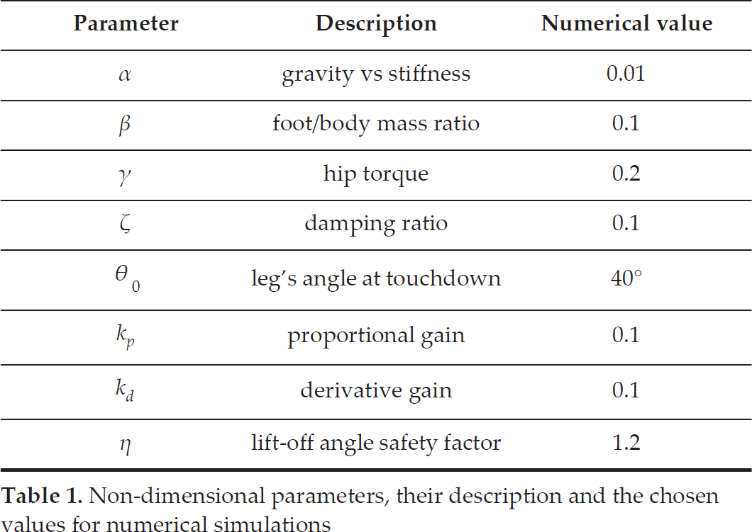
In this section, numerical simulation results of the TDMF-SLIP model under representative parameter values are presented and analysed. Special focus is given to analysing the influence of the friction coefficient μ on the emergence of different types of periodic solutions and on their performance. In order to minimize the number of independent parameters, the system's dynamics is normalized by the characteristic time of $\sqrt{m/k}$ , the leg's free length l₀ and body mass m. Four non-dimensional parameters are defined as $\alpha =\frac{mg}{k{l}_0}$ , $\beta =\frac{m_f}{m}$ , $\gamma =\frac{{\tau }_0}{k{l}_0^2}$ and $\zeta =\frac{c}{2\sqrt{mk}}$ . The chosen numerical values of all non-dimensional parameters throughout for simulations are given in Table 1. While the choice of values of $\alpha \mathrm{,}\beta \mathrm{,}\gamma \mathrm{,}\delta \mathrm{,}\zeta$ and ${\theta }_0$ has some physical and biological relevance, the parameters $k_p\mathrm{,}{k}_d\mathrm{,}\eta$ - related to the control law - were chosen by trial and error in order to achieve a reasonably fast convergence of the leg's motion during flight to the desired trajectory, which is similar to that of the massless leg model.

Table 1.

Non-dimensional parameters, their description and the chosen values for numerical simulations

Parameter	Description	Numerical value
α	gravity vs stiffness	0.01
β	foot/body mass ratio	0.1
γ	hip torque	0.2
ζ	damping ratio	0.1
θ 0	leg's angle at touchdown	40°
kp	proportional gain	0.1
kd	derivative gain	0.1
η	lift-off angle safety factor	1.2

5.1. Classifying different types of periodic solutions with slippage

We now present a classification of different types of periodic solutions of the TDMF-SLIP under slippage. These periodic solutions are demonstrated via numerical simulation results under representative values of friction coefficient μ, where the values of all other non-dimensional parameters are taken from Table 1. Simulations of the system's hybrid dynamics were conducted by event-driven numerical integration of the equations of motion (8), using the ode45 command in $\text{MATLAB}{}^{TM}$ . For each value of μ, stable periodic solutions were found by numerically searching for fixed points of the Poincaré map $\Pi$ . Since the system now has four degrees of freedom $q$ , the state vector $x=(q\mathrm{,}\stackrel{·}{q})$ is eight-dimensional and the Poincaré section at the centre-of-mass apex point $\stackrel{·}{y}{}_c=0$ is seven-dimensional, while reduction due to energy conservation is no longer possible. Each periodic solution that contains a single impact can be classified according to the sequence of stick/slip states during the stance phase from touchdown to lift-off. Thus, each type of solution can be classified as a word from the alphabet $\{-\mathrm{,0,}+\}$ , which corresponds to the sign of slippage velocity $\stackrel{·}{x}$ and thus represents a sequence of states of negative slip, sticking or positive slip, respectively.

Figure 5 shows simulation results of a stable periodic solution of the TDMF-SLIP under high friction of $\mu =10$ . Plots of the normalized heights of the foot $y(t)$ and centre-of-mass $y_c(t)$ along a full period from apex to apex are shown in Figure 5(a), where t is the normalized time. The two vertical dashed lines enclose the time duration of the stance phase. Figure 5(b) plots the normalized leg length $r(t)$ and the leg angle $\theta (t)$ in degrees along a full period from apex to apex. One can see that $r(t)$ converges to its free length of 1 (normalized by l₀) under the influence of damping and that it is compressed to values smaller than 1 during stance phase. Due to the action of the controlled hip torque τ in (12), the angle $\theta (t)$ converges to the desired value ${\theta }_0$ after apex time and to the constant value of $\eta {\theta }_{LO}$ after lift-off. Figure 5(c) plots the foot's tangential velocity $\stackrel{·}{x}(t)$ . One can see that the impact results in immediate sticking $\stackrel{·}{x}{}^{+}=0$ , which persists for almost the entire duration of the stance phase. It can also be seen that $\stackrel{·}{x}(t)$ changes continuously but not smoothly at the beginning and end of the period, due to the discontinuous change in the control law (12) at apex time. Figure 5(d) plots the ground force ratio $f_x/f_y$ during the stance phase. One can see that when the normal force f_y tends to zero directly before lift-off, this ratio reaches its lower bound of $-\mu$ and a very short period of positive slippage evolves, followed by immediate lift-off. The ‘×’ at the left end of the plot denotes the ratio of impulses $F_x/F_y$ at the impact. Since this ratio is above $-\mu$ , condition (4) is satisfied and the impact results in sticking, $\stackrel{·}{x}{}^{+}=0$ . Thus, this periodic solution can be classified as type ‘ $0+$ ’. The vertical dash-dotted line denotes the mid-stance time at which $\theta =0$ , where the switch in the control law in (11) imposes a discontinuous jump in the ground reaction forces.

Figure 5.

Plots of a periodic solution for $\mu =10$ : (a) Normalized heights of the foot $y(t)$ and centre-of-mass $y_c(t)$ . (b) Normalized foot length $r(t)$ and leg angle $\theta (t)$ in degrees. The vertical dashed lines enclose the time of stance phase. (c) Plot of the foot's tangential velocity $\stackrel{·}{x}(t)$ , where the jump to zero indicates a sticking impact. (d) Plot of the force ratio $f_x/f_y$ during the stance phase. Upon lift-off, this ratio reaches the bound $-\mu$ , resulting in a short episode of slippage. The vertical dash-dotted line indicates mid-stance $\theta =0$ , where the actuation torque τ vanishes. The ‘ × ’ at the left end denotes the ratio of impulses $F_x/F_y$ at the impact.

When the friction coefficient μ is decreased, condition (4) is no longer satisfied and the impact results in positive slip. As an example, Figure 6 shows the simulation results of a stable periodic solution under friction coefficient $\mu =1.2$ . Figure 6(a) plots the tangential foot velocity $\stackrel{·}{x}(t)$ . The plot indicates that $\stackrel{·}{x}$ does not vanish due to impact; hence, the stance phase begins with a short episode of positive slippage followed by sticking and another brief slippage right before lift-off. Thus, this periodic solution can be classified as type ‘ $+0+$ ’. The ratio of tangential to normal contact forces during stance phase $f_x/f_y$ is shown in Figure 6(b), where the dashed line for which $f_x=-\mu f_y$ denotes slip, while the solid line denote sticking. One can observe that the transition from slip to stick involves discontinuity of the contact forces, while the converse transition (directly before liftoff) does not.

Figure 6.

Plots of a periodic solution for $\mu =1.2$ : (a) The foot's tangential velocity $\stackrel{·}{x}(t)$ , where the jump indicates a slipping impact and the dashed line indicates slippage. (b) Plot of the force ratio $f_x/f_y$ during the stance phase. Right after impact, the dashed line at $-\mu$ indicates slippage, followed by sticking (solid curve) and another brief slippage right before lift-off. The vertical dash-dotted line indicates mid-stance $\theta =0$ , where the actuation torque τ vanishes.

When μ is further decreased, another interesting type of stable periodic solution evolves, which is classified as $\text{'}+0-0+\text{'}$ . As an example, Figure 7 plots simulation results for $\mu =0.6$ , where Figure 7(a) plots the foot's tangential velocity $\stackrel{·}{x}(t)$ , while Figure 7(b) plots the contact force ratio $f_x/f_y$ during the stance phase. The periodic solution now consists of three phases of slippage separated by two phases of sticking. Upon further decrease of μ, the two episodes of sticking gradually shrink until they disappear. For $\mu =0.43$ , the tangential velocity $\stackrel{·}{x}(t)$ during the stance phase is plotted in Figure 8(a). This periodic solution is classified as type ‘ $+0-$ ’, where the latter phase of sticking disappears and liftoff occurs after negative slip. For $\mu =0.2$ , the tangential velocity $\stackrel{·}{x}(t)$ during the stance phase is plotted in Figure 8(b). This periodic solution is classified as type ‘ $+-$ ’, where the first phase of sticking also disappears and the foot slips during the entire stance phase. A reversal of the slippage direction occurs during stance, which implies a discontinuous jump in the contact forces and a nonsmooth change of velocities. When μ is decreased further, no qualitative change in the periodic solution is observed; however, numerical simulations for $\mu <0.1$ become extremely sensitive and no periodic solutions can be numerically obtained.

Figure 7.

Plots of a periodic solution for $\mu =0.6$ . (a) The foot's tangential velocity $\stackrel{·}{x}(t)$ , where the jump indicates a slipping impact and the dashed line indicates slippage. (b) Plot of the force ratio $f_x/f_y$ during the stance phase. The vertical dash-dotted lines indicate mid-stance $\theta =0$ , where the actuation torque τ vanishes.

Figure 8.

Plots of the foot's tangential velocity $\stackrel{·}{x}(t)$ during the stance phase of a periodic solution for (a) $\mu =0.43$ and (b) $\mu =0.2$ . Solid line indicates sticking, while dashed lines indicate slippage. The vertical dash-dotted lines indicate mid-stance $\theta =0$ , where the actuation torque τ vanishes.

5.2. Influence of friction coefficient on performance

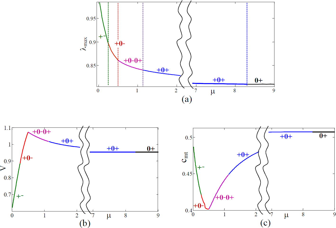
We now analyse the influence of changes in the coefficient of friction μ on three key characteristics of periodic solutions: stability, average speed and energetic efficiency. Stability is determined by the magnitude of the eigenvalues ${\lambda }_i$ of the linearization of the Poincaré map $\Pi$ , where the condition ${\lambda }_{max}=\text{max}\left\{\left|{\lambda }_i\right|\right\}<1$ has to be satisfied for stability. The linearization matrix $D\Pi (x{}^{*})$ was obtained by numerically computing the Poincaré map under perturbations of the state $x$ about $x{}^{*}$ , in small variations of each state variable. Figure 9(a) plots the maximal eigenvalue magnitude ${\lambda }_{max}$ as a function of μ. The dashed vertical lines denote critical values of μ where the periodic solution undergoes a transition in its type, and the different types are shown as labels near the curve. The range $\mu \in [\mathrm{2,7}]$ is cut out from the plot in order to improve the visibility of lower values of μ, since the periodic solution type remains as ‘ $+0+$ ’ within this range, while the value of ${\lambda }_{max}$ changes monotonically. It can be seen that the stability of the periodic solution degrades as μ is decreased and slippage evolves. For values of μ below 0.3, computation of $D\Pi (x{}^{*})$ became numerically sensitive, since perturbations about $x{}^{*}$ led to solutions with a second impact immediately after lift-off. This sensitivity can be mitigated by better tuning of the control parameters $\eta \mathrm{,}{k}_p\mathrm{,}{k}_d$ of the actuation torque τ in (12) for the flight phase. This insignificant tuning is not discussed in this work.

Figure 9.

(a) Plot of the maximal linearization eigenvalue ${\lambda }_{max}$ of periodic solutions as a function of the friction coefficient μ. The vertical dashed lines denote transitions between different types of periodic solutions, which are indicated by the text labels. (b) Average speed V as a function of μ. (c) Mechanical cost of transport $c_{mt}$ of the periodic solutions as a function of μ.

The average speed of a periodic solution is defined as $V=\mathrm{\Delta }x/T$ , where $\mathrm{\Delta }x$ is the step length and T is the step's period time. Figure 9(b) plots V as a function of μ, where the range $\mu \in [\mathrm{2,7}]$ is cut out from the plot. Remarkably, it can be seen that decreasing μ results in an increase in the average speed V, due to the evolution of forward slippage, which is not stopped by the impact. Maximal speed for the given parameter values is obtained at $\mu \approx 0.5$ , which provides roughly a $12\%$ increase compared to the speed at no-slip solutions for large friction. When μ is decreased below 0.5 the speed drops again, since the periodic solutions of type ‘ $+0-$ ’ involve negative slip prior to lift-off, which cancels the effect of the positive slip after impact. When μ is decreased below 0.2, where solution type ‘ $+-$ ’ evolves, the negative slip becomes dominant and the speed V drops sharply.

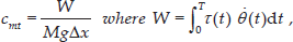
The energetic efficiency of legged locomotion is evaluated based on the mechanical cost of transport [20, 32, 47], which is the mechanical work per distance, defined as

$c_{mt}=\frac{W}{Mg\mathrm{\Delta }x}whereW={\displaystyle {\int }_0^T}\tau (t)\stackrel{·}{\theta }(t)\mathrm{d}t\mathrm{,}$

(13)

W is the mechanical work expended by the hip torque actuation during a full period and $Mg=(m+m_f)g$ is the total weight. This is analogous to measuring “gallons per mile” in cars, where lower values of $c_{mt}$ correspond to greater energetic efficiency. Figure 9(c) plots the value of the mechanical cost of transport $c_{mt}$ of periodic solutions as a function of μ, where the range $\mu \in [\mathrm{2,7}]$ is cut out from the plot. Remarkably, it can be seen that decreasing the friction coefficient reduces $c_{mt}$ substantially for all values of μ, in spite of the added energy dissipation due to slippage. The reasons for this increase are twofold: first, the onset of slipping impact, which does not fully stop the forward velocity results in increasing the step length $\mathrm{\Delta }x$ . Second, energy losses due to slipping impact are significantly smaller than those of sticking impact, at which the tangential velocity is always stopped. Optimal energetic efficiency is obtained at $\mu \approx 0.5$ , which provides roughly a $25\%$ decrease in $c_{mt}$ , compared to the value at no-slip solutions for large friction. When μ is decreased below 0.5, the duration of slip phases becomes large and the resulting dissipation causes an increase in energy expenditure W. Moreover, the onset of negative slip decreases the step length $\mathrm{\Delta }x$ and hence, the overall effect is that of increasing $c_{mt}$ .

5.3. Discussion

We now discuss the results of the numerical simulations presented above. First, the observation that periodic solutions with slippage due to low friction are less stable (larger $\lambda {}_{max}$ ) compared to those with large friction is in good agreement with the observed results in [18, 19] for models of passive dynamic walking, except for the fact that in these works, stability was lost ( $\lambda {}_{max}>1$ ) below a critical value of μ. Note that lower linearization eigenvalues only indicate faster convergence to the periodic solution under small perturbations. Perhaps a more useful measure of stability will be in the region of attraction, which was not studied here, due to its high dimensional complexity in systems with many degrees of freedom. An important observation from the numerical simulations is that some of the numerically computed linearization eigenvalues of $D\Pi (x{}^{*})$ were very close to zero, a fact that indicates that the effective dimension of the Poincaré map can be reduced. While the dimension of the state vector $x$ is 8 (four degrees of freedom, coordinates $x_m\mathrm{,}{y}_m\mathrm{,}x\mathrm{,}y$ or $x_c\mathrm{,}{y}_c\mathrm{,}r\mathrm{,}\theta$ and their velocities), the Poincaré section at apex is defined by the constraint $\stackrel{·}{y}{}_c=0$ and hence, its dimension is 7. However, in all types of periodic solutions under different values of μ, four out of the seven numerically computed eigenvalues of $D\Pi (x{}^{*})$ were very small, in the order of ${10}^{-3}-{10}^{-5}$ . The reason for this is the presence of hidden constraints on the hybrid dynamics, which are more evident if one chooses different Poincaré sections along the periodic solutions. According to the explanations in [62], the rank of the Poincaré map is determined by the Poincaré section with the smallest dimensions. If one chooses a Poincaré section at post-impact states, where $y=0$ and $\stackrel{·}{y}>0$ , the assumption of inelastic impact imposes an additional constraint on the state space, $\stackrel{·}{y}{}^{+}=0$ . Moreover, under sticking impact, which occurs in periodic solutions of type ‘ $0+$ ’, the constraint $\stackrel{·}{x}{}^{+}=0$ is also imposed. That is, the Poincaré section at post-impact states has an effective dimension of 6 for slipping impact and 5 for sticking impact. On the other hand, if one chooses a Poincaré section at pre-impact states, where $y=0$ and $\stackrel{·}{y}<0$ , other constraints are imposed by the chosen control law at flight phase (12), which forces convergence of the foot angle $\theta (t)$ towards its desired value of ${\theta }_0$ prior to touchdown, as seen in Figure 5(b). Moreover, the leg's damping attenuates the two-mass oscillations and the distance $r(t)$ also converges towards its free length l₀ (normalized value of 1) as also seen in Figure 5(b). This implies that the state vector $x$ at the pre-impact Poincaré section is very close to satisfy the constraints $\theta {}^{-}={\theta }_0\mathrm{,}$ $r^{-}=l_0$ and ${\dot{\theta }}^{-}={\stackrel{·}{r}}^{-}=0$ . Therefore, according to the theory in [62], the effective rank of the Poincaré map drops from 7 to 3, as corroborated by the numerical results of the present study.

Finally, another interesting observation is that for some intermediate ranges of μ, the average forward speed V increases due to slippage, which contrasts the results obtained in [19] for the actuated compass biped walking under slip-stick transitions. A possible explanation for this difference is the specific choice made for the control law in [19], which used a reference trajectory with small step length that reduces walking speed. Nevertheless, the increase in energetic efficiency due to the presence of slipping impact in the periodic solution is in good qualitative agreement with the results in [19].

6. Conclusion

In this paper, we analysed a generalized version of the SLIP model that incorporates the effects of Coulomb friction and foot slippage by adding a foot mass, linear damping and controlled torque actuation. The influence of the friction coefficient on different types of periodic solutions with different contact transitions was analysed. It was found that periodic solutions under low friction and foot slippage are less stable in terms of linearization eigenvalue magnitude. On the other hand, for some intermediate ranges of μ, average speed and energetic efficiency were significantly increased in the presence of slippage, mainly due to slipping impact which does not completely stop the foot's tangential velocity and thus results in smaller losses of energy and forward speed, compared to a no-slip periodic solution. For the chosen parameter values, an optimal value of friction coefficient that maximizes the average speed and energetic efficiency is $\mu \approx 0.5$ , which is a practically achievable value.

We now briefly discuss the limitations of this work and propose possible directions for future extension of the research. First, it is obvious that the proposed complex model of TDMF-SLIP lacks much of the elegance and simplicity of the original SLIP model, mainly due to the increase in dimensionality and the necessity of arbitrarily specifying a particular control law for the hip torque during flight. Nevertheless, the reduction in dimensionality of the Poincaré map due to four nearly-zero eigenvalues suggests that this model can be simplified into a lower-dimensional model. One may consider a reduced model, in which the details of two masses and torque actuation are taken into account only during the stance phase, while during flight phase, the two masses are approximated as a single rigid body, whose angle θ is prescribed kinematically upon touchdown. This model has a three-dimensional Poincaré section at the pre-impact state, which can be further reduced to two dimensions by ignoring the x coordinate, due to invariance of the dynamics with respect to it. This proposed reduction, which is currently under our investigation, results in a much simpler model that is amenable to more thorough analysis of the influence of the system's parameters on dynamic behaviour and performance.

Second, it is planned to systematically fit the parameters of the TMDF-SLIP model in order to match measured results from the legged motion of animals where significant foot slippage is observed, in order to test the biological relevance of the model.

Third, it is important to incorporate different methods of actuation into the model and test their influence on the modification of gaits in order to minimize foot slippage, or for harnessing slippage to improve performance. In addition, incorporation of control strategies developed for various generalizations of the SLIP model into the TMDF-SLIP model in order to test their interaction with possible foot slippage on varying terrains is a challenging open problem. In particular, it is worth revisiting the concept of swing leg retraction (SLR) [52]. Inspired by legged animal locomotion, the SLR concept involves retraction of the leg angle θ during flight according to a linear time profile, $\theta (t)={\theta }_a-{\omega }_0(t-t_a)$ , where t_a is the time at apex and ${\theta }_a\mathrm{,}{\omega }_0$ are given constants. The SLR method is known to significantly enhance the stability of the periodic solutions of the SLIP model and to also add robustness with respect to uncertainties in ground height [54]. Since this control concept affects the foot's velocity upon touchdown, it will be interesting to analyse its interaction with friction constraints and possible foot slippage. Finally, our model can be extended by considering more detailed models for contact, friction and slippage; cf. [22, 45].