Sage Journals: Discover world-class research

Abstract

During the past three decades, PCIs – process capability indices – have inspired hundreds of pages of scientific research. The trade-off between simplicity and precision in reproducing an overall process quality prediction is both the reason behind the criticism for Cp and Cpk and the motive for their widespread use. Indeed, their strength in simplifying the assessment of a process control status compensates for some of the statistical shortcomings largely recognized in the literature, amongst which is the normality assumption. Hence, this article aims at overcoming the main statistical problems of Cp and Cpk indices by proposing a new indicator, still compliant with the traditional PCIs approach, but applicable for cases of non-normal processes while being simple to implement and easy to interpret. The proposed indicator is composed of three sub-indices, each related to a specific process characteristic: how the process is repeatable, how much the data distribution is skewed about the mean value and how much the process data comfortably lies between the specifications limits. On top of this, a specific parameter allows designers or quality engineers to modify the index value range in order to finetune the effect of the cost of Taguchi's loss function. The article presents the theoretical structure of the new indicator and an extensive numerical test on several different processes with different distributions upon multiple specification limit combinations, along with a comparison to the Cpk index, in order to demonstrate how the new index provides a clearer indication of the process criticalities.

Keywords

Process Capability Process Performance PCI Statistical Process Control

1. Introduction

1.1 Literature review on PCIs

The importance of process capability indices (PCIs) mirrors their strategic role in the quality control activities, especially in the manufacturing processes. PCIs provide a numerical value of whether or not a manufacturing process is capable of meeting a specified level of tolerances. In fact, their structure creates a relation between process data indices (mean, median standard deviation, etc.) and the specification limits, upper specification limit (USL) and lower specification limit (LSL) [1,2]. Among the most widespread PCIs is the Cp [3,4,5], which is meant to be a measure of overall process precision related to manufacturing tolerances [4,5]. However, Cp cannot provide an assessment of process centring or targeting; this information is given by Ca index [6]:

C p = \frac{U S L - L S L}{6 σ}; C a = 1 - \frac{| μ - m |}{d}

where μ indicates the process mean; σ, the process standard deviation; d, half the tolerance width; and m, the mid value between USL and LSL. Ca is an index that measures the degree of the process centring with respect to the specification limits. In order to show process accuracy and its distance from the nearest specification limit, Cpk index was introduced [7]:

C p k = Min {\frac{USL - μ}{3 σ}, \frac{μ - LSL}{3 σ}} = C p \times C a = \frac{d - | μ - m |}{3 σ}

Cpk fails, however, to tell where the process mean is located in the tolerance range and, as is shown later, its use is inappropriate with asymmetric distributions.

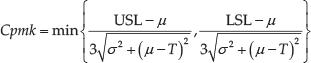
In spite of this, Cp and Cpk are widely recognized as adequate indices to measure quality standards and to lead improvements in manufacturing industry, especially where the reduction of the process variability is considered the primary driver for quality progress [2]. Their simplicity is the reason for recent complex improvements of Cp and Cpk formulas not finding fertile ground for manufacturing implementation. Indeed, the literature reports several other PCIs, spun off from Cp and Cpk formulas: in the late 1980s, Hsiang and Taguchi [8,9] introduced the Cpm:

C p m = \frac{USL - LSL}{6 \sqrt{σ^{2} + {(μ - T)}^{2}}}

Then Cpmk followed [10,11]:

C p m k = min {\frac{USL - μ}{3 \sqrt{σ^{2} + {(μ - T)}^{2}}}, \frac{LSL - μ}{3 \sqrt{σ^{2} + {(μ - T)}^{2}}}}

Cpmk index can also be expressed using Ca and Cp [2] and is one of the most well-known PCIs [12]. Specifically, it shows some advantages compared with Cp, Cpk and Cpm:

Cpk considers the process yield, whereas Cpm considers process loss and variation from the target. Since Cpmk is a combination of Cpk and Cpm, it has the advantages of both Cpk and Cpm [13].

Since Cpmk provides more information about the location of the process mean, it is more sensitive than Cpk and Cpm to the deviation of the departure of process mean (being Cpmk the least sensitive) [10] and its reaction to the changes in process variations is faster [14].

In 1995, Vannman [11] proposed a unified approach with a complex superstructure Cp (u, v), where Cp, Cpk, Cpm and Cpmk represent specific cases and can be obtained by setting u and v parameters.

In the past 25 years, the properties and the applicability of these indices have been extensively investigated [15, 16, 17, 18, 19, 20, 21, 22, 23, 24,25, 26, 27, 28]. As a result, the shared opinion is that these indices are adequately reliable when used with normally distributed processes; however, these can be more or less inappropriate for measuring and evaluating the quality of non-normal processes. Several studies illustrate the poor performance of the normally based capability indices as a predictor of process fallout, when the process is not normally distributed [2,7,29,30,31]. Consequently, some authors suggested specific modifications in Cpk and Cp formulas for increasing their applicability to non-normal processes, for example:

Pearn et al. [10] suggested to replace 6σ in the Cp formula with 6θ, ‘where θ is chosen so that the capability is not affected to a large extent by the shape of the distribution at end.’

Clements et al. [32] proposed to replace 6σ in the Cp formula with the length of the interval between upper and lower 0.135 percentage points of the given distribution.

Wright [33] recommended to introduce a corrector factor in Cpmk denominator to consider distribution skewness.

Pearn et al. [34] proposed to modify the Cp (u, v) superstructure [11] in order to be applied to processes with arbitrary distributions.

Deleryd [35] suggested to tune u and v parameters in Cp (u, v) to deal with skewness.

Finally, in 2001, a new index Spmk was proposed [36] to take into account process variability and proportion of nonconformity for non-normal processes.

However, all of these proposals tend to introduce additional mathematical hurdles on top of the Cp structure, failing to address one of the most critical requisites of a PCI index: simplicity. Indeed, the success of PCIs mainly raise from their ability to decode the complex statistical reality into simple words that direct workers and process leaders or managers can quickly understand. Considering that not all workers in the manufacturing industry master statistics, the indices structures must be as close as possible to their understanding. For example, this is one of the reasons behind the widespread choice in industry of sampling PCIs values into intervals (e.g., 1 < Cpk < 1.33) rather than presenting them with their bare absolute values in order to quickly obtain a mark, linked with a certain risk prediction. Consequently, PCIs should be able to quickly and clearly tell the factors that influence performances.

1.2 The design of PCIs

The study of a manufacturing process capability implies four main steps:

Collecting process data;

Evaluating the distribution shape of process data;

Creating and interpreting the control charts;

Calculating the overall capability coefficients and indices.

The last step is when the process status passes from an operative control phase to a managerial one. Indeed, it is the step where a capability study becomes a status for a risk assessment and acquires the role of performance predictor. Historically, PCIs evolution influenced (i), e.g., through the definition of sampling strategies as well as (ii) and (iii) inspiring several quality control handbooks and special application environments development.

By merging this approach with the management's interest on process status and the risk assessment role of PCIs, it is possible to list three main improvement areas:

Non-normality has to be recognized and evaluated by a PCI as a lack of predictability; this statement is demonstrated by the fact that current PCI's correlation between their score and the process yield starts from the assumption that the process data are normally distributed.

Cp and Cpk and all their variations are not significant if analysed alone. Together, they are able to describe a risk in terms of quality assurance but, currently, this risk is not deployable into independent sub-indices.

The quality loss included in the Cpm and Cpmk denominator represents a key improvement because it succeeds in considering the cost of the distance between the process mean and the target value. However, it is not possible to evaluate it independently from other performance aspects related to distribution features.

After so many detailed studies, Cp and Cpk index family may not be further improvable. Spmk index [36] resulted to be more effective in terms of dealing with non-normal processes, but it has lost the characteristic of simplicity that was one of the key factors for the success of Cp and Cpk indices.

2. Proposed index structure

This article proposes a new PCI with the following characteristics:

Simple, to be read from managers to line teams as well.

Unhampered by any theoretical distribution assumption.

Able to treat non-normality as a penalty factor in terms of predictability.

Composed of independent sub-indices, each able to describe a distribution feature, including quality loss.

Coupled with the managerial concept of risk assessment through the use of percent values, where 100% is the score related to the absence of risk.

Last point recalls the OEE – overall equipment effectiveness – index structure [37]: OEE is a simple index used in Operations Management to measure equipment effectiveness loss in manufacturing industry; it is designed to support the workforce in bottom-up improvement actions, being composed of three independent percent parameters: easy to understand, to compare, to bucket into slots, and to drive the path to further calculations or useful breakdowns.

Here, the aim is similar: the proposed index has the following structure:

P S H = P \times S \times H

where P, S and H are three independent percent sub-indices and their multiplication returns the PSH index (PuSH in its fancy alias). The three sub-indices respond to three key distribution characteristics:

How the process is repeatable, that is, how much the process data distribution shows a small variance (P = Pulse).

How much the data distribution is skewed about the mean value (S = Shape).

How much the process data comfortably fit inside the specification limits, that is, is far from the boundaries (H = Housing).

In the next paragraphs, each sub-index is defined and explained. Henceforth, on top of the previously defined symbols, the following notation will be used, with reference to the parameters in Figure 1.

Figure 1.

Variables used in the PSH index structure

2.1 Pulse

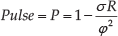
The first sub-index is P (Pulse), which aims to evaluate the variability of the distribution. Taking the clue from Cp, it compares the distribution's variability with the specification range:

P = 1 - \frac{σ R}{φ^{2}}

The structure of the P sub-index can be easily interpreted with reference to Figure 2. As P tends to 100%, the more the process is repeatable and reproducible. P = 1 indicates the Dirac delta distribution, and this value can only be asymptotically pursued. Analogously, P could theoretically reach negative values when the distribution range and the standard deviation are much higher than φ. However, this situation hardly occurs in industrial processes. For low values of P, one should analyse the bigger deviation samples and identify – typically, through pro techniques and root-cause approaches – the eventual specific causes that generated the outlier data.

Figure 2.

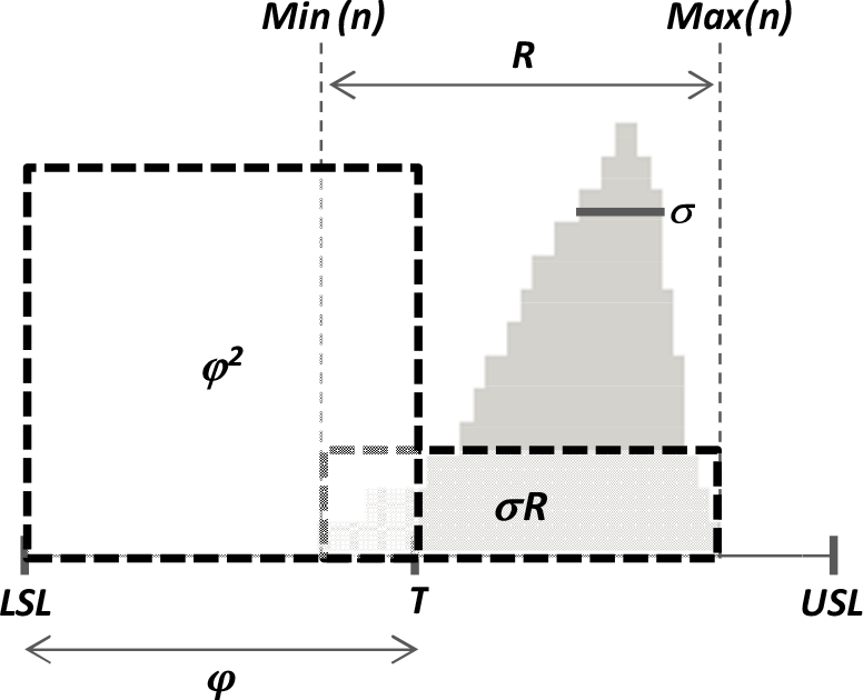
Variables used in the P index structure

2.2 Shape

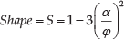
The second sub-index describes the risk to deal with a non-normal data distribution. Clearly, in order to pursue a simplicity target, S could not be based on a statistical normality test but on an indicator of the distribution symmetry. The index takes inspiration from the second Pearson's index, and its formula follows:

S = 1 - 3 {(\frac{α}{φ})}^{2}

where

α = | 3 (μ - M_{e}) |

and M_e indicates the median of the sample distribution. As said, the Shape index recalls Pearson's index [38]:

| P_{2} | = \frac{| 3 (μ - M_{e}) |}{σ}

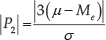
Following the risk assessment concept of PCIs, we may consider that asymmetry could be a risk if it gets large with respect to the specification tolerance. Thus, in a risk assessment index, the distance between median and mean should be correlated to the tolerance.

After taking into consideration an asymmetric worst case, which gives a | P₂ | = 1.2, we have set our index on the foundation that a risky process for a normal standard distribution (Cp = 1) has σ = (USL–LSL)/6. Finally, we have designed the Shape formula in order to let it evaluate the worst case described above with a score of 50%. Figure 3 could graphically explain the Shape formula.

Figure 3.

Variables used in the S index structure

2.3 Housing

The third sub-index is H (Housing). As mentioned in the introduction, in Cp and Cpk (especially in Cpm and Cpmk), the position of the mean is not evaluated by an independent index, but it participates in the calculation of the PCI's score. On the contrary, the H formula evaluates the position of the distribution with respect to the specification limits:

H = 1 - {(\frac{δ}{φ - C})}^{4}

where δ = | μ – T | and C = kσ

Accordingly, H = 1 indicates the distribution's range is centred within the specification tolerances interval, and this means that the process is probably performing in the best condition to avoid an out-of-tolerance part. The more δ increases, the more the risk to generate points out of bounds increases as well. When H = 0, the distribution's mean is even centred on (USL – kσ) or (LSL + kσ).

The H sub-index walks on the path ploughed by Taguchi [8] in trying to consider the loss in products worth when one monitored characteristic deviates from a target value. Here, the tolerance impact on performance can be specified acting on k parameter, as shown in Figure 4, which depicts three cases of different values of k=0, 1, 2 on a tolerance interval of ±5, for a normal standard distribution. The parameter k is to be set by designers, considering which effect this characteristic brings to the product's overall performance. In the following numerical experiments, k=1 will be used to represent an average situation.

Figure 4.

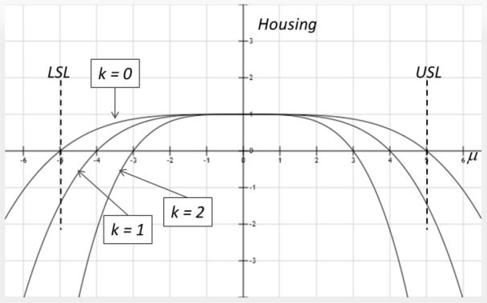
k parameter used in the H index structure

For low values of H, process teams should focus on input material status, equipment settings, parameters set up, and so on. Indeed, shifting a distribution centre is easier than acting on its shape, in terms of variability and skewness.

3. Validation of PuSH index

In the validation phase, PuSH index has to achieve the eligibility to be a solid alternative to the current PCIs. To reach this goal, a preliminary theoretical validation is required to compare Cp and Cpk with PuSH index, both on specific theoretical distributions and on several sampling cases in different scenarios.

3.1 Test with theoretical process distributions

A set of theoretical distributions have been generated to evaluate Cp, Cpk and PuSH results:

Three non-normal distributions have been chosen: Gamma, Beta and Lognormal distributions.

Each distribution has five different configurations where their fundamental parameters are changed to obtain different skewness degrees.

Each configuration is tested considering 11 couples of specification limits, calculated in order to obtain, respectively, 11 constant Cpk values.

Every single process is evaluated with three indices: PuSH, Cpk and Q (the latter indicating the percentage within the limits or yield [2]).

Figures 5, 6 and 7 show the theoretical distributions used in the test along with a table indicating the values of their typical parameters in each different configuration. The parameter values have been chosen to obtain significantly different distribution shapes and skewness degrees.

Figure 5.

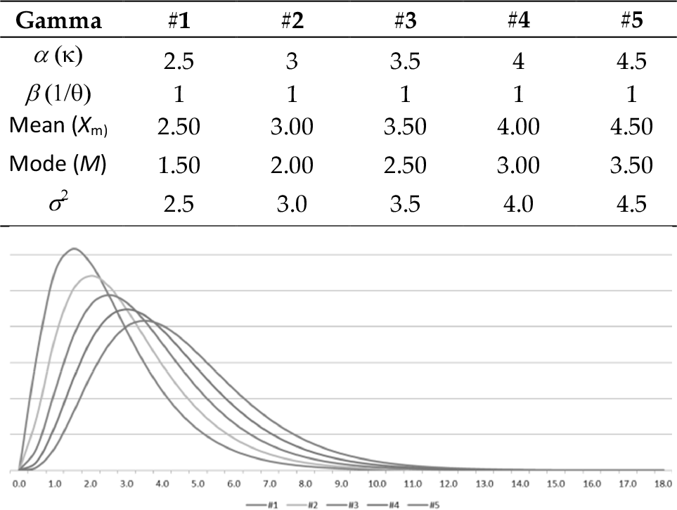
Gamma distributions

Figure 6.

Beta distributions

Figure 7.

Lognormal distributions

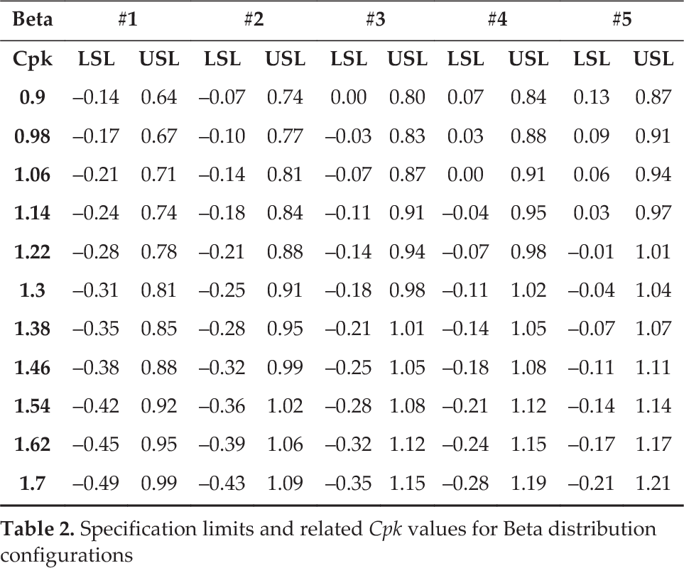
Thus, 3 distributions tested on 5 configurations and 11 sets of different limits are obtained, hence 165 cases. Given that the value range cannot be computed for theoretical distributions, in order to compute PuSH index we have assumed that minimum and maximum values in each distribution are described by the 1st and the 99th percentile. Tables 1, 2, 3 show all the configuration limits computed per each distribution and each configuration (thus all the cases), along with the related Cpk value.

Table 1.

Specification limits and related Cpk values for Gamma distribution configurations

Gamma	#1		#2		#3		#4		#5
Cpk	LSL	USL	LSL	USL	LSL	USL	LSL	USL	LSL	USL
0.9	−1.77	6.77	−1.68	7.68	−1.55	8.55	−1.40	9.40	−1.23	10.23
0.98	−2.15	7.15	−2.09	8.09	−2.00	9.00	−1.88	9.88	−1.74	10.74
1.06	−2.53	7.53	−2.51	8.51	−2.45	9.45	−2.36	10.36	−2.25	11.25
1.14	−2.91	7.91	−2.92	8.92	−2.90	9.90	−2.84	10.84	−2.75	11.75
1.22	−3.29	8.29	−3.34	9.34	−3.35	10.35	−3.32	11.32	−3.26	12.26
1.3	−3.67	8.67	−3.75	9.75	−3.80	10.80	−3.80	11.80	−3.77	12.77
1.38	−4.05	9.05	−4.17	10.17	−4.25	11.25	−4.28	12.28	−4.28	13.28
1.46	−4.43	9.43	−4.59	10.59	−4.69	11.69	−4.76	12.76	−4.79	13.79
1.54	−4.80	9.80	−5.00	11.00	−5.14	12.14	−5.24	13.24	−5.30	14.30
1.62	−5.18	10.18	−5.42	11.42	−5.59	12.59	−5.72	13.72	−5.81	14.81
1.7	−5.56	10.56	−5.83	11.83	−6.04	13.04	−6.20	14.20	−6.32	15.32

Table 2.

Specification limits and related Cpk values for Beta distribution configurations

Beta	#1		#2		#3		#4		#5
Cpk	LSL	USL	LSL	USL	LSL	USL	LSL	USL	LSL	USL
0.9	−0.1	4 0.64	−0.07	0.74	0.00	0.80	0.07	0.84	0.13	0.87
0.98	−0.1	7 0.67	−0.10	0.77	−0.03	0.83	0.03	0.88	0.09	0.91
1.06	−0.2	1 0.71	−0.14	0.81	−0.07	0.87	0.00	0.91	0.06	0.94
1.14	−0.2	4 0.74	−0.18	0.84	−0.11	0.91	−0.04	0.95	0.03	0.97
1.22	−0.2	8 0.78	−0.21	0.88	−0.14	0.94	−0.07	0.98	−0.01	1.01
1.3	−0.3	1 0.81	−0.25	0.91	−0.18	0.98	−0.11	1.02	−0.04	1.04
1.38	−0.3	5 0.85	−0.28	0.95	−0.21	1.01	−0.14	1.05	−0.07	1.07
1.46	−0.3	8 0.88	−0.32	0.99	−0.25	1.05	−0.18	1.08	−0.11	1.11
1.54	−0.4	2 0.92	−0.36	1.02	−0.28	1.08	−0.21	1.12	−0.14	1.14
1.62	−0.4	5 0.95	−0.39	1.06	−0.32	1.12	−0.24	1.15	−0.17	1.17
1.7	−0.4	9 0.99	−0.43	1.09	−0.35	1.15	−0.28	1.19	−0.21	1.21

Table 3.

Specification limits and related Cpk values for Lognormal distribution configurations

LogN	#1		#2		#3		#4		#5
Cpk	LSL	USL	LSL	USL	LSL	USL	LSL	USL	LSL	USL
0.9	1.26	4.29	1.03	4.55	0.80	4.82	0.57	5.10	0.32	5.40
0.98	1.13	4.42	0.88	4.70	0.63	5.00	0.37	5.30	0.10	5.62
1.06	0.99	4.55	0.72	4.86	0.45	5.18	0.16	5.51	−0.13	5.85
1.14	0.86	4.69	0.57	5.02	0.27	5.35	−0.04	5.71	−0.35	6.07
1.22	0.72	4.82	0.41	5.17	0.09	5.53	−0.24	5.91	−0.58	6.30
1.3	0.59	4.96	0.25	5.33	−0.09	5.71	−0.44	6.11	−0.80	6.53
1.38	0.45	5.09	0.10	5.48	−0.27	5.89	−0.64	6.31	−1.03	6.75
1.46	0.32	5.23	−0.06	5.64	−0.45	6.07	−0.84	6.51	−1.25	6.98
1.54	0.18	5.36	−0.21	5.80	−0.62	6.25	−1.04	6.71	−1.48	7.20
1.62	0.05	5.50	−0.37	5.95	−0.80	6.43	−1.25	6.92	−1.70	7.43
1.7	−0.08	5.63	−0.53	6.11	−0.98	6.60	−1.45	7.12	−1.93	7.65

On each case, the PuSH index has been computed. Figures 8, 9 and 10 show the results comparing the process yield (Q) in percentage with Cpk and PuSH values. The aspect to be evaluated is the indices pattern with respect to the Q curve: the more accurately an index pattern follows the yield curve, the better the index capability describes the process performance.

Figure 8.

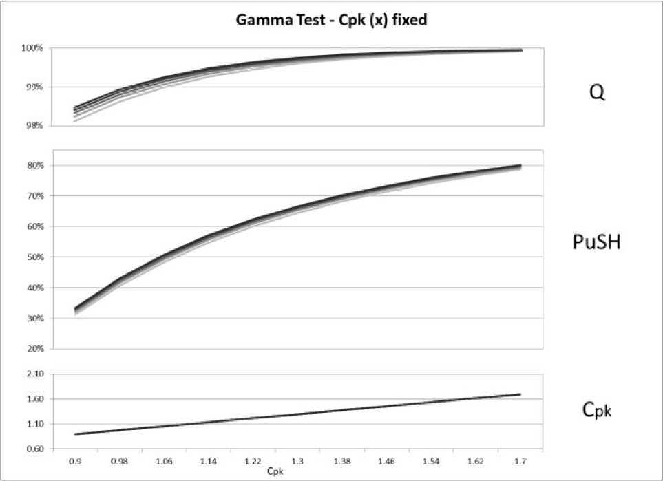
Comparison between yield (Q), PuSH and Cpk trends on Gamma distribution configurations

Figure 9.

Comparison between yield (Q), PuSH and Cpk trends on Beta distribution configurations

Figure 10.

Comparison between yield (Q), PuSH and Cpk trends on Lognormal distribution configurations

First, the PuSH indicator resulted to be able to return different values according to distribution skewness: indeed, changing the distribution configuration (i.e., asymmetry) PuSH curve shifts up or down, while Cpk always returns the same line. Secondly, PuSH seems to follow the trend of Q more precisely, returning a concave curve, whereas Cpk returns a straight line, which is particularly evident with the Gamma and Lognormal cases.

3.2 Test with discrete distributions

PuSH has also been validated with a set of data samples ad hoc generated to describe realistic situations of both normal and non-normal processes. The 12 distributions shown in

Figure 11 (each of 200 samples) were us e d to compute both PuSH and Cpk with 12 sets of different limits configuration (scenarios), hence 144 cases.

Figure 11.

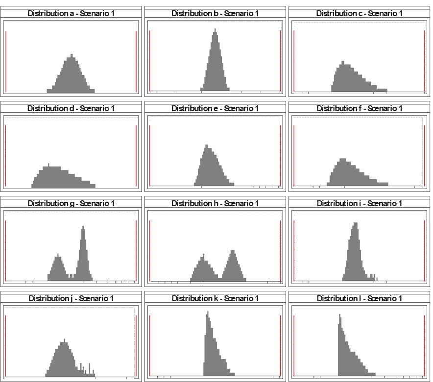
Generated distributions, shown in their first scenario (centred)

The x-axis ranges from 0 to 10. The 12 scenarios specification are defined by assigning different USL and LSL couples, as shown in Figure 12.

Figure 12.

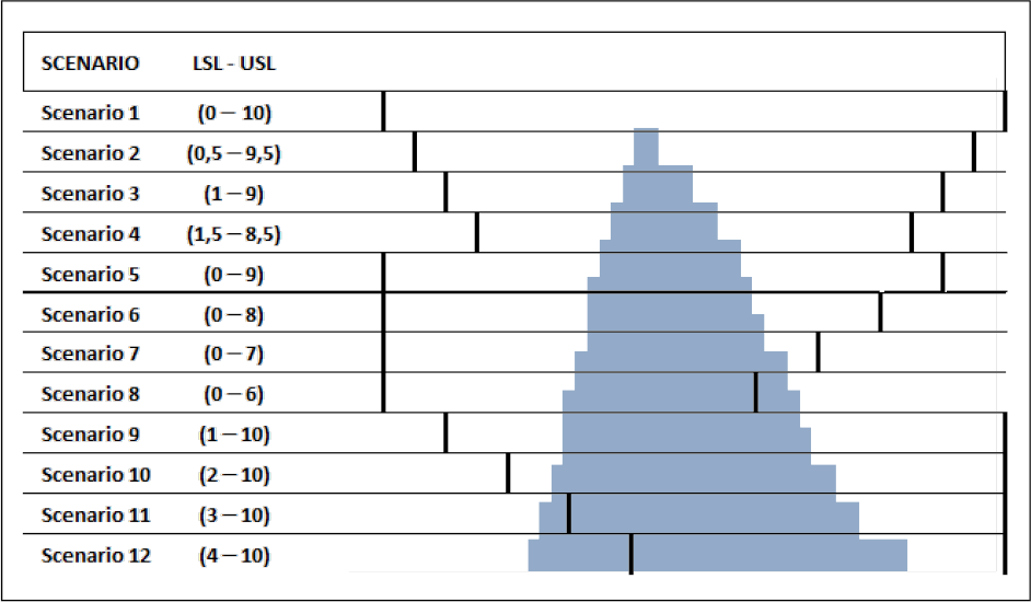
Different scenarios obtained changing the specs limits position

Table 4 shows the different values of PuSH and Cpk for each of the 144 cases.

Table 4.

Testing results

Scenario#		1	2	3	4	5	6	7	8	9	10	11	12
A	Cpk	2.29	2.06	1.83	1.60	1.83	1.37	0.90	0.44	1.87	1.41	0.95	0.49
A	PuSH	87.3%	84.4%	80.4%	74.7%	84.4%	79.6%	67.4%	22.9%	84.4%	79.8%	69.1%	30.6%

B	Cpk	3.65	3.26	2.88	2.50	3.26	2.49	1.73	0.96	2.88	2.11	1.34	0.58
B	PuSH	91.3%	89.4%	86.6%	82.6%	89.4%	86.4%	80.4%	60.0%	89.3%	85.3%	73.9%	31.4%

C	Cpk	1.50	1.33	1.16	0.99	1.50	1.22	0.88	0.54	1.16	0.82	0.48	0.14
C	PuSH	75.2%	69.8%	62.6%	52.6%	69.9%	62.6%	51.9%	29.6%	69.2%	57.9%	28.0%	−65.9%

D	Cpk	1.17	1.03	0.89	0.75	1.17	1.09	0.81	0.53	0.89	0.61	0.32	0.04
D	PuSH	70.1%	63.6%	54.8%	42.8%	63.9%	55.3%	43.4%	23.2%	62.1%	44.9%	−3.0%	−138.7%

E	Cpk	2.41	2.16	1.90	1.65	2.15	1.65	1.14	0.63	1.90	1.40	0.89	0.38
E	PuSH	89.0%	86.4%	83.0%	78.0%	86.4%	82.8%	75.1%	48.5%	86.3%	81.4%	66.9%	10.7%

F	Cpk	1.39	1.24	1.08	0.93	1.39	1.08	0.77	0.46	1.08	0.77	0.46	0.15
F	PuSH	71.7%	65.7%	57.5%	46.4%	65.7%	57.5%	45.2%	19.7%	65.2%	53.6%	24.9%	−57.8%

G	Cpk	1.56	1.40	1.24	1.07	1.24	0.91	0.58	0.26	1.38	1.05	0.72	0.40
G	PuSH	64.7%	57.4%	47.9%	35.4%	57.3%	46.6%	27.4%	−10.8%	57.4%	47.7%	32.8%	6.5%

H	Cpk	1.29	1.16	1.02	0.89	1.02	0.75	0.48	0.21	1.15	0.88	0.60	0.33
H	PuSH	69.5%	63.1%	54.6%	43.1%	62.9%	52.5%	28.6%	−41.9%	63.1%	54.2%	38.9%	0.0%

I	Cpk	3.14	2.81	2.47	2.13	2.94	2.27	1.59	0.92	2.47	1.79	1.11	0.44
I	PuSH	93.2%	91.7%	89.5%	86.4%	91.7%	89.4%	84.6%	66.4%	91.5%	87.5%	74.0%	18.4%

J	Cpk	1.89	1.69	1.49	1.29	1.69	1.29	0.89	0.50	1.49	1.09	0.69	0.30
J	PuSH	82.6%	78.7%	73.4%	65.9%	78.7%	73.2%	62.7%	31.2%	78.6%	71.6%	53.6%	−9.6%

K	Cpk	3.04	2.73	2.42	2.11	2.53	1.91	1.29	0.67	2.42	1.80	1.18	0.57
K	PuSH	92.1%	90.2%	87.7%	84.1%	90.2%	87.3%	79.7%	49.8%	90.2%	86.9%	77.2%	38.2%

L	Cpk	2.06	1.82	1.57	1.33	2.06	1.79	1.31	0.83	1.57	1.09	0.61	0.13
L	PuSH	86.5%	83.4%	79.2%	73.2%	83.5%	79.4%	73.1%	58.9%	82.6%	73.5%	44.5%	−61.6%

Before presenting the analysis of certain selected scenarios, it is necessary to define some thresholds for the PuSH indicator, in order to cluster the results for supporting decisions. For this purpose, we can use a correlation diagram to set up slots to bucket the PuSH's results, by taking the clue from Cpk thresholds, currently used in manufacturing management. Indeed, in statistical process control, a key characteristic should have Cpk > 1.33. The Cpk > 1.67 represents the process requirement for critical characteristics, while Cpk < 1 describes an undesired process performance. Thus, Cpk slots are as follows:

Critical (high risk, ‘red flag’): Cpk < 1

Average (medium risk, ‘yellow flag’): 1 ≤ Cpk < 1.33

Good (low risk, ‘light green flag’): 1.33 ≤ Cpk < 1.67

Optimal (very low risk, ‘green flag’): Cpk ≥ 1.67

The correlation diagram in Figure 13 shows a good correlation between Cpk and PuSH.

Figure 13.

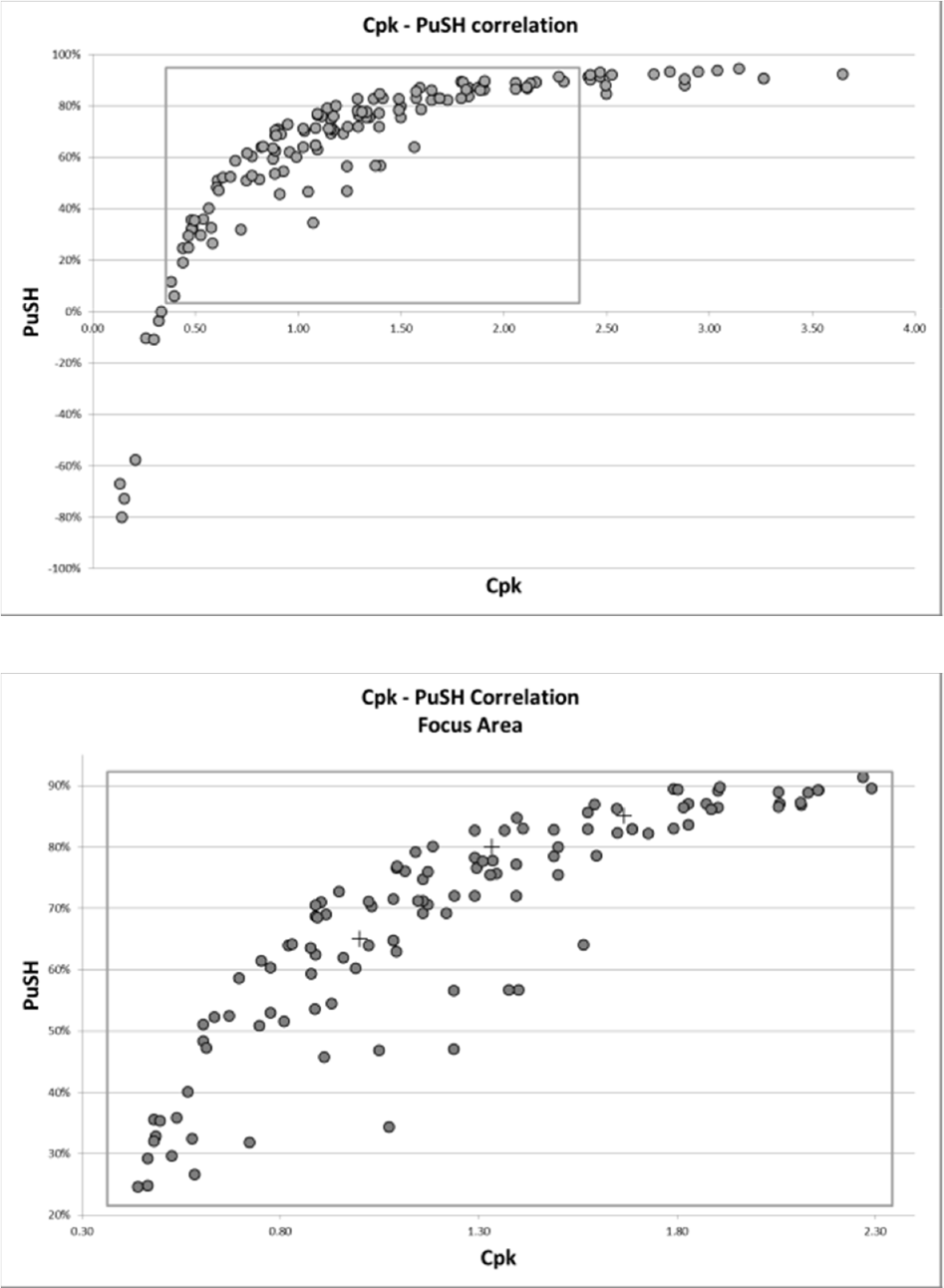
Correlation diagrams between PuSH and Cpk

The PuSH-Cpk equivalent values can be found in correspondence to Cpk thresholds on the regression curve drawn on the correlation diagram of A and B normal distributions (considering that Cpk is not suitable for non-normal distributions), as shown in Figure 14.

Figure 14.

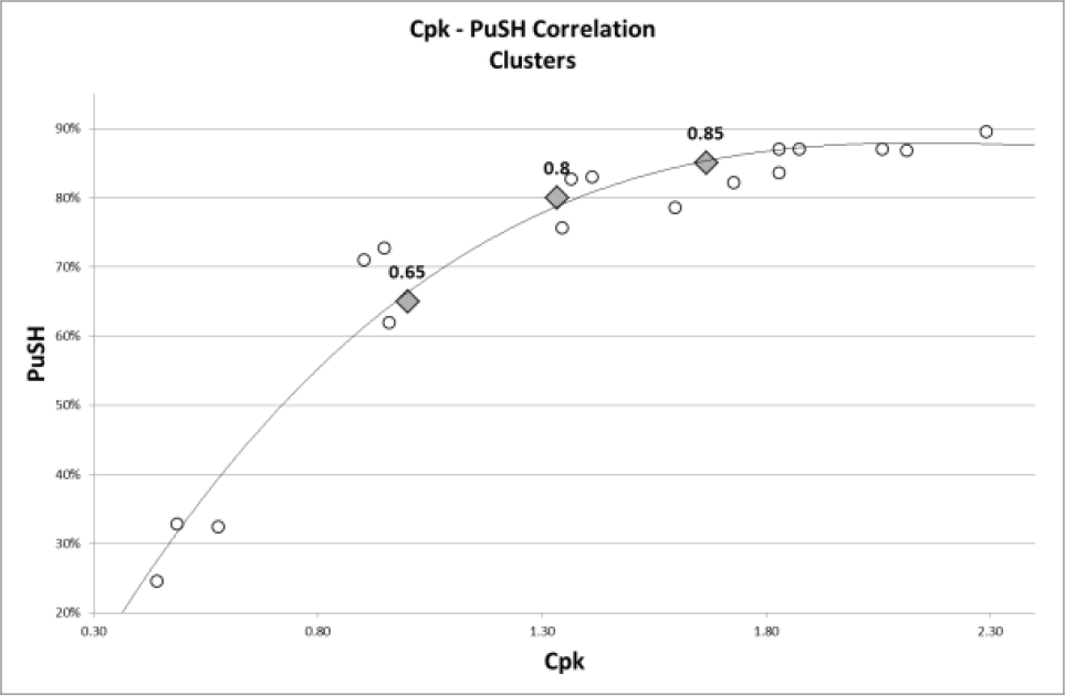
Regression on Gaussian distributions for PuSH thresholds

Hence we have:

Critical (high risk, ‘red flag’): PuSH < 65%

Average (medium risk, ‘yellow flag’): 65% ≤ PuSH < 80%

Good (low risk, ‘light green flag’): 80% ≤ PuSH < 85%

Optimal (very low risk, ‘green flag’): PuSH ≥ 85%

These thresholds describe the PuSH slots used in the examples in the following paragraph.

3.2.1 Similar Cpk, different PuSH

The following examples show how Cpk index fails to discriminate between two different cases, while PuSH provides a clearer indication on the process criticalities. Case f5 and e10 are two asymmetric distributions: the first is a centred distribution characterised by a large range and thick asymmetry, whereas the second is more symmetric and tight, but slightly uncentred, as in Figures 16 and 17. Figure 15 graphically shows that Cpk cannot discriminate between the two cases (Cpk = 1.39 and 1.40, indicating a low risk process with ‘green’ rating), while PuSH only ranks e10 as ‘good’ (PuSH = 84.7%) while f5 is classified ‘average’ (PuSH = 72%).

Figure 15.

Processes with similar Cpk score, but different PuSH

Figure 16.

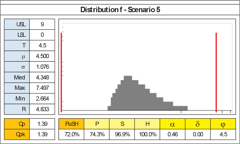
f5 details

Figure 17.

e10 details

This difference, in terms of process overall evaluation, is due to three peculiar characteristics:

Pulse considers the distribution's range, and f5 value range is greater.

Shape considers the asymmetry, and f5 value is clearly more asymmetric than e10.

Housing is meant to underline when the mean gets closer to the specification limits. For k =1, the shifting of e10 distribution decreases H value to 98.1%.

In summary, the large asymmetric tail – which can be considered as clue for a higher risk process – penalizes f5 in PuSH index, whereas e10's relative centring is sufficient to rank it as a ‘good’ process. Recalling that k parameter (in C = kσ) is the one to act on in order to reduce the process acceptance tolerances, in case the requirements for this specific process were stricter, the designer would have set k to a higher value. For example, if e10 was evaluated with k=3, the Housing sub-index would have returned H=85.7, thus the overall process ranking would have been ‘average’ (PuSH = 74.0).

This example clearly shows how PuSH index provides much more detailed indications on the process with respect to Cpk.

3.2.2 The effect of k parameter

Recalling that the 144 cases have been evaluated using k=1 in computing the Housing sub-index, the effectiveness of k parameter is best shown comparing what happens with cases a3 (k=1), a6 (k=1) and a6 (k=3), shown in Figures 18, 19 and 20.

Figure 18.

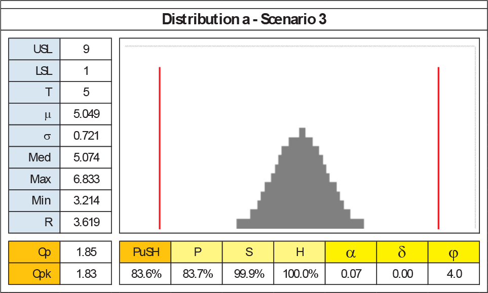
Distribution a3 details

Figure 19.

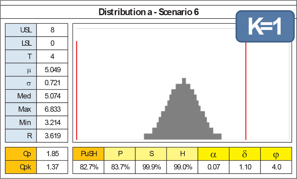
Distribution a6 details and k = 1

Figure 20.

Distribution a6 details and k = 3

This nice bell-shaped normal process has been evaluated with a perfect centring between the specifications limits (a3) versus a significant drifting (a6): as expected, both Cpk and PuSH index decrease (Cpk from 1.83 to 1.37 and PuSH from 83.6% to 82.7%). First, the PuSH's overall index reduction is driven only by the H sub-index's decreasing. Second, one may argue that the penalization resulting from the distribution shifting in the PuSH index is, however, not sufficient. Indeed, the k parameter can tune this effect: in Figure 20, a6 case has been evaluated with k=3: now, PuSH indicator reaches 74.7%. Thus, from a6 case, the delta is now 8.9% instead of 0.9%. In summary, k gives designers or quality engineers the chance to increase or decrease the attention to the cost of Taguchi's loss function.

3.2.3 Similar Cpk, different PuSH

Analogously, there are examples of a couple of cases when Cpk seem to discriminate better than PuSH: let us compare b8 with g1, both shown in Figures 21, 22 and 23. These two cases present similar PuSH (62.0% and 64.1%) but different Cpk (respectively 0.96 and 1.56). b8 is a nice tight bell, indicating a precise process; however, its mean is largely shifted towards the USL and a significant part of its right tail is out of the specification limit, which is a clear unacceptable situation. Indeed, both Cpk and PuSH rank the process as ‘high risk’, red flag. On the contrary, g1 is a perfectly centred process with a point distribution relatively far from the specification limits. As to Cpk, the process is good (Cpk = 1.56), whereas PuSH stays on the same value as before: high risk.

Figure 21.

Processes with similar PuSH score, but different Cpk

Figure 22.

b8 details

Figure 23.

g1 details and the bimodal shape effect on PuSH

Indeed, the Shape sub-index downgrades the overall index because of asymmetry: g1 is a bimodal distribution, and this characteristic is perceived by PuSH index. Both distribution indicate risky processes, for different reasons: b8 has mainly problems in terms of Housing (78.3%) while g1 for its Shape (75%). From the industrial point of view, it is hard to say which distribution one would prefer to face: indeed, they are not comparable in terms of effect on product performance (g1 is surely better than b8), but bimodality is the typical symptom of a potential problem because the process may not be under control. While Cpk definitely opts for the bimodal distribution, PuSH still indicates a potential risk in both cases. Without watching the distribution histograms (in massive data analysis in industrial contexts, decisions are taken only relying on indices), it would have been impossible to identify g1 subtle characteristic only using the Cpk index. On the contrary, despite the similar score of b8, PuSH clearly points out that there may be a problem with g8: eventually, something strange, not known and hard to predict. Thus, at least this leads to further analyses and the subsequent choice of improvement actions.

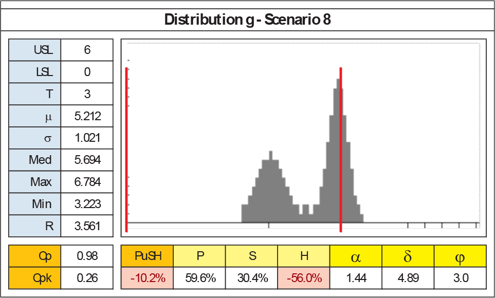
3.2.4 Negative PuSH

Like Cpk, PuSH value also could reach below zero. However, PuSH results are more severe: while negative values in Cpk indicate that the mean is out of the tolerance range, negative values in PuSH are reached even if the mean is too close to the specification limits, within a distance of C =kσ, while P and S are positive.

Figure 24 shows g8 case, where H= −56%. When μ proximity to the limits can menace the final performance (defined through designers' k), Housing becomes negative.

Figure 24.

g8 details and the negative Housing situation

P and S could be negative too, but in extreme and abnormal situations (σR greater than half-squared tolerance, median very far from the mean, and so on).

3.2.5 More on Housing: the design assurance

Let us consider the example shown in Figure 25: it is a very narrow bell, extremely close to the LSL (μ=2 and USL-LSL = 9–1 = 8), with Cp = 6.44 anda Cpk = 1.61. Cpm and Cpmk (0.44 & 0.11) recognize the quality loss, by acting on the formulas denominator.

According to the Cpk score, it is a very good process, despite its dramatic shifting. It is clear how the quality loss to produce far from the target value T is considered not crucial.

According to the Cpmk score (0.11), it is a bad process, because of its dramatic shifting. It explains the reason behind the positive comments about Cpmk previously explained.

For PuSH it is a bad process too, because of the Housing index.

Figure 25.

Example of quality loss

Cpmk [8] partially solves this issue, replacing σ with $\sqrt{σ^{2} + {(μ - T)}^{2}}$ in the denominator of the Cpk formula: the more μ is far from T, the more Cpk score decreases. It means that Cpmk can receive and feel the quality loss, but it does not give the chance to weight this loss in a design phase. There may be industrial contexts where the example of Figure 25 entails the risk of huge losses, or other contexts where quality may not be affected by such a distribution position. On the contrary, in PuSH index, designers could set k=0 for characteristics that do not have a quality performance loss, in terms of system and customer expectations. If so, Housing gets very permissive. Differently, they may set k=3 or higher values for characteristics where μ must be as much as possible closer to T. Housing gives a great opportunity to designers in an early phase of the product development and production: it lets them define the k factor for each characteristic, before any process and production scores. In other words, the designer is the subject who initially defines how much ‘critical’ is the quality loss with respect to the desired value, or the target value. Thus, if scoring a process, which must be able to produce within the specification limits, is part of quality assurance, Housing index describes the previously weighted risk for producing far from the desired value: this is a design assurance activity.

4. Conclusions

We have presented a new easy-to-use process capability index, applicable to cases of non-normal processes, with an improved potential to describe process characteristics in a more accurate way than Cpk. The proposed brand new PCI is P.S.H., or alternatively called PuSH, which is the result of the multiplication of 3% sub-indices:

P u S H = P \times S \times H

where P (Pulse) evaluates the distribution spreading with respect to a given specified tolerance:

P u l s e = P = 1 - \frac{σ R}{φ^{2}}

S (Shape) evaluates the confidence level of dealing with a symmetric set of data:

S h a p e = S = 1 - 3 {(\frac{α}{φ})}^{2}

H (Housing) evaluates the centring of the data set with respect to the specification limits, and it includes a parameter, k, in C = kσ, by taking the clue from Taguchi's quality loss theory. The factor k, in contrast to the Cpm formula, lets the designer decide how sensitive the desired performance is with respect to the process centring:

Housing = H = 1 - {(\frac{δ}{φ - C})}^{4}

Cpk and PuSH have been compared on three theoretical distributions (Gamma, Beta, Lognormal) with five different degrees of skewness each. Results show that PuSH is able to distinguish the skewness of each distribution and more precisely follows the yield trend with respect to Cpk. Then Cpk and PuSH have been tested on 144 hypothetical processes, combining 12 different discrete distributions (10 out of 12 were non-normal) with 200 samples each and on 12 different specification limits scenarios. As a result, the following slots have been set from the correlation of both indices scores, computed on normal discrete distributions (Table 5):

Table 5.

Score thresholds for Cpk and PuSH

	Cpk	PuSH
Critical, ‘red flag’	<1.00	<65%
Average, ‘yellow flag’	1.00< x<1.33	65%< x<80%
Good, ‘light green flag’	>1.66	>85%
Optimal, ‘green flag’	1.33< x<1.66	80%< x<85%

According to these thresholds, the 144 processes scores are summarized in Table 6.

Table 6.

Number of processes in each score bucket

	Cpk	PuSH
Critical, ‘red flag’	52 (36.1%)	57 (39.6%)
Average, ‘yellow flag’	30 (20.8%)	34 (23.6%)
Good, ‘light green flag’	20 (13.9%)	14 (9.8%)
Optimal, ‘green flag’	42 (29.2%)	39 (27.0%)
Total	144	144

A deeper analysis of these numbers shows that 36 scores are assigned to different buckets. In other words, a different risk rate is assigned to these processes. Table 7 shows these 36 different assignments.

Table 7.

Comparison of Cpk and PuSH different scores

		PuSH
		Critical	Average	Good	Optimal
Cpk	Critical	−	6

	Average	8	−	2

	Good	3	8	−	3

	Optimal			6	−

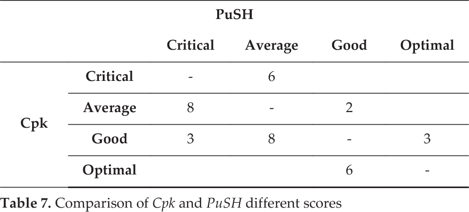
The processes evaluations from PuSH being less critical than Cpk are shown above the diagonal in Table 7. Vice versa below the diagonal. Results show that PuSH returned more strict values than Cpk in 25 cases out of 144, mainly because of the presence of large distribution range and asymmetry, both aspects not considered in Cpk calculations. On the contrary, Cpk returned more strict values than PuSH in 11 cases out of 144, and this only due to the k=1 parameter setting used in this test in the H sub-index. Considering that k parameter is to be set by designers according to the relative importance one wants to assign to the quality loss function, this result does not represent a critical issue.

To sum up, by comparing selected cases, the article showed that PuSH – through its sub-indices – is able to provide analysts with much more accurate information with respect to Cp and Cpk. Thanks to its sub-indices – Pulse, Shape and Housing – PuSH is able to quickly tell:

If shape and skewness, considered as risks in terms of predictability, may affect the process risk assessment;

If data centring represents an improvement issue, independent of the process repeatability;

When a tiny tail or a large values range should be considered as a source of risk;

Which values should be pursued for each sub-index in order to achieve the required overall PuSH performance.

On top of being easy to calculate and interpret, PuSH, with its Housing sub-index may present designers with the opportunity to set the undesired quality and performance loss in an early phase. These results helped in a preliminary assessment of PuSH reliability and precision, leading the way to an extensive testing phase on real manufacturing cases and further research on k parameter setting and tuning in industrial contexts. This extensive testing phase will also allow risk assessment slots to be set for the PuSH sub-indices.

Thanks to these results, the PuSH logic supports in a more effective way the overall process evaluation by management, and, furthermore, gives process teams more information about the risk, evident by Pulse, Shape and Housing sub-indices.

References

Kotz

and Johnson

N. L.

, Process capability indices, London, UK: Chapman & Hall, 1993.

Chien-Wei

Pearn

W. L.

and Kotz

, An overview of theory and practice on process capability indices for quality assurance, International Journal of Production Economics 117 (2009), 338–359, 2009.

Juran

J. M.

, Quality control handbook, 3rd ed., New York, NY: McGraw-Hill, 1974.

Sullivan

L. P.

, Targeting variability – A new approach to quality, Quality Progress 17 (7), 15–21, 1984.

Kane

V. E.

, Process capability indices, Journal of Quality Technology 18 (1), 41–52, 1986.

Pearn

W. L.

Lin

G. H.

and Chen

K. S.

, Distributional and inferential properties of process accuracy and process precision indices, Communication in Statistics: Theory & Methods 27 (4), 985–1000, 1998.

Somerville

S. E.

and Montgomery

D. C.

, Process capability indices and non-normal distributions, Quality Engineering 9, 305–316, 1996–1997.

Hsiang

T. C.

and Taguchi

, A tutorial on quality control and assurance – The Taguchi methods, Las Vegas, NV: ASA Annual Meeting, 1985.

Chan

L. K.

Cheng

S. W.

and Spiring

F. A.

, A new measure of process capability Cpm, Journal of Quality Technology 20 (3), 162–175, 1988.

10.

Pearn

W. L.

Kotz

and Johnson

N. L.

, Distributional and inferential properties of process capability indices, Journal of Quality Technology 24 (4), 216–231, 1992.

11.

Vannman

, A unified approach to capability indices, Statistica Sinica 5, 805–820, 1995.

12.

Abdolshah

, Fuzzy process capability indices: A review, World Applied Sciences Journal 16 (12), 1734–1740, 2012.

13.

Jessenberger

and Weihs

, A note on the behavior of Cpmk with asymmetric specification limits, Journal of Quality Technology 32 (4), 440–443, 2000.

14.

, Assessing process capability based on Bayesian approach with subsamples, European Journal of Operational Research 184 (1), 207–228, 2008.

15.

Zhang

Stenback

and Wardrop

, Interval estimator of process capability index Cpk, Communication in Statistics: Theory & Methods 19, 4455–4470, 1990.

16.

Owen

and Borrego

, Lower confidence limits on process capability indices based on the range, Communications in Statistics: Simulation & Computation 19 (1), 1–24, 1990.

17.

Kushler

and Hurley

, Confidence bounds for capability indices, Journal of Quality Technology 24, 188–195, 1992.

18.

Nagata

and Nagahata

, Approximation formulas for the lower confidence limits of process capability indices, Okayama Economic Review 25, 301–314, 1994.

19.

Chen

and Hsu

, The asymptotic distribution of the process capability index Cpmk, Communication in Statistics: Theory & Methods 24, 1279–1291, 1995.

20.

Tang

Than

and Ang

, A graphical approach to obtaining confidence limits of Cpk, Quality & Reliability Engineering International 13, 337–346, 1997.

21.

Zimmer

Hubele

and Zimmer

, Confidence intervals and sample size determination for Cpm, Quality & Reliability Engineering International. 17, 51–68, 2001.

22.

Vannman

, Distribution and moments in simplified form for a general class of capability indices, Communications in Statistics: Theory & Methods 26, 159–179, 1997.

23.

Wright

, The probability density function of process capability index Cpmk, Communication in Statistics: Theory & Methods 27 (7), 1781–1789, 1998.

24.

Wright

, The cumulative distribution of process capability index Cpm, Statistics & Probability Letters, 47, 249–251, 2000.

25.

Hoffman

, Obtaining confidence intervals for Cpk using percentiles of the distribution of Cp, Quality and Reliability Engineering International 17 (2), 113–118, 2001.

26.

Zimmer

and Hubele

, Quantiles of the sampling distribution of Cpm, Quality Engineering 10, 309–329, 1997.

27.

Pearn

and Shu

, Lower confidence bounds with sample size information for Cpm applied to production yield assurance, International Journal of Production Research 41 (15), 3581–3599, 2003.

28.

Kotz

and Lovelace

, Process capability indices in theory and practice, London, UK: Arnold, 1998.

29.

English

J. R.

and Taylor

, Process capability analysis – A robustness study, International Journal of Production Research 31, 1621–1635, 1993.

30.

Castagliola

, Evaluation of non-normal process capability indices using Burr's distributions, Quality Engineering 8, 587–593, 1996.

31.

Johnson

Kotz

and Pearn

, Flexible process capability indices, Pakistan Journal of Statistics 10 (1), 23–31, 1994.

32.

Clements

, Process capability calculations for nonnormal distributions, Quality Progress 22 (9), 95–100, 1989.

33.

Wright

P. A.

, A process capability index sensitive to skewness, Journal of Statistical Computation & Simulation 52, 195–203, 1995.

34.

Pearn

W. L.

and Chen

K. S.

, Capability indices for non-normal distributions with an application in electrolytic capacitor manufacturing, Microelectronics Reliability 37 (12), 1853–1858, 1997.

35.

Deleryd

, Process capability indices in theory and practises, Licentiate Thesis, Division of Quality Technology and Statistics, Lulea University of Technology, 1996.

36.

Jann-Pygn

and Cherng

G. D.

, A new process capability index for non-normal distributions, International Journal of Quality & Reliability Management 18 (7), 762–770, 2001.

37.

Nakajima

, Introduction to TPM: Total productive maintenance, Cambridge, MA: Productivity Press, 1988.

38.

Pearson

, Notes on regression and inheritance in the case of two parents, Proceedings of the Royal Society of London 58, 240–242, 1895.

A Proposal for a Management-Oriented Process Capability Index

Abstract

Keywords

1. Introduction

1.1 Literature review on PCIs

1.2 The design of PCIs

2. Proposed index structure

2.1 Pulse

2.2 Shape

2.3 Housing

3. Validation of PuSH index

3.1 Test with theoretical process distributions

3.2 Test with discrete distributions

3.2.1 Similar Cpk, different PuSH

3.2.2 The effect of k parameter

3.2.3 Similar Cpk, different PuSH

3.2.4 Negative PuSH

3.2.5 More on Housing: the design assurance

4. Conclusions

References