A Method Based on Bottleneck-Linear Assignment for Forming Complex Transport Formations

Abstract

Cooperative transportation using multi-robots is a significant challenge in robotics. For the problem, each robot is required, in general, to reach a different task-point to form a transport formation, where all the task-points are determined according to the shape of the transported object and the number of robots. A method based on bottleneck-linear assignment is proposed to form complex transport formations. First, the optimal paths from each robot to all the task-points are calculated by a two-direction path algorithm, which is developed in this paper as the core of the task-points' assignment. Second, in order to optimize the travelling paths of the robots and the time taken to establish the formation, a bottleneck-linear assignment strategy is presented to assign the task-points for the robots. Finally, an improved artificial moment motion controller makes each robot move along a sub-optimal path to reach its task-point. Simulations indicate that the proposed method is feasible and efficient.

1. Introduction

Cooperative transportation by multi-robots is an interesting and challenging problem in robotics. Much attention has been paid on its study [1–5] as it holds the promise of a wide range of applications. For example, for a factory in a serious fire, cooperative transportation by multi-robots can be used to rescue workers in coma and to remove any obstacles along exit passageways and so forth.

The grasping-based method and caging-based method are two important methods addressing the problem. Under the grasping-based method, a force-closure or form-closure condition is achieved by the robots' contacts. Under these conditions, the robot mechanism can resist any external force and generate acceleration for a transported object [2, 6, 7, 8]. In most cases, robots are the only source of grasp forces. When external forces acting on the transported object, such as gravity and friction, are used together with contact forces to produce force-closure, this is a situation of conditional force-closure. In [9, 10], conditional force-closure is used for object-pushing and other tasks.

Under the caging-based method, the object-closure condition is always achieved [2, 8, 11–14]. Under this condition, the object has some freedom to move, and the contact between the object and the robotic mechanism need not to be maintained. As a result, the motion planning and control of each robot become simpler, and the coordination among the robots becomes easier.

Under the methods for the cooperative transportation problem, all the robots in the group are required, in general, to approach the object to form a transport formation that satisfies certain conditions and constraints, such as an object-closure condition and the limitation of the manipulating force of each robot. For instance, in [8, 13, 14], a method based on an object-closure condition is presented. Its first step is to form a transport formation as noted above.

In [13], a method based on potential fields is presented for forming transport formations with the advantages of low computational burden and scalable numbers of robots. However, the method is unable to form a desired transport formation if the object is not star-shaped [13]. The paths travelled by the robots and the duration to establish formations are not optimized either, even though this may be a significant aspect.

In [15], a method based on handling-points (“task-points” in this paper) is proposed for forming complex transport formations, and its general steps are as follows. First, a host robot computes all the task-points according to the number of robots and the shape of the object, and assigns each robot a different task-point. When the first step is successfully completed, each robot will move towards its task-point so that a desired formation can be established. The method presents an important idea for forming transport formations, i.e., all task-points are easy to calculate according to the number of robots and the shape of the object and so forth. If each robot can be assigned to a suitable task-point and move along a sub-optimal path to reach the task-point, then the paths travelled by robots and the time taken to establish formations can be optimized. Furthermore, a desired formation can be always achieved, no matter how many robots exist and how complex the object is. However, the method takes the line segment between a robot and a task-point as the optimal path between them, and each robot is forced to move along a line segment toward its task-point without considering the object and other robots. As a result, when some of the line segments are blocked by the object or by other robots, the method becomes unfeasible.

Up to now, most of the existing works on transport formations do not consider how to optimize the paths travelled by robots and the time taken to establish formations, and few existing methods can guarantee that a desired formation can be formed in cases where the shape of the object is very complex.

Motivated by the limitations noted above and the basic idea of the method in [15], a new method based on bottleneck-linear assignment is developed in this paper for forming complex transport formations, and which can be viewed as an improvement of the method in [15]. The main contributions of the proposed method are presented below.

1. Inspired by the idea of Dijkstra's algorithm [16, 17] and the fact that all task-points are placed around and close to the object, a two-direction path algorithm is developed for computing the optimal paths from each robot to all the task-points. Via the algorithm, a matrix about the optimal paths from the robots to the task-points is obtained which is the foundation for assigning the task-points.

2. To optimize the paths travelled by the robots and the time taken to establish formations, a bottleneck-linear assignment strategy is proposed to assign each robot a reasonable task-point. The proposed assignment inherits the advantages of bottleneck assignment and general linear assignment [18] while avoiding their shortcomings. As a result, it performs much better than bottleneck assignment and general linear assignment.

3. To decrease the computational burden of the artificial moment motion controller presented in [19–21], the methods for attractive segments and attractive points are improved. As a result, when the controller is used to make each robot move safely along a sub-optimal path towards its task-points, the performance in real-time of the controller is improved.

The rest of this paper is organized as follows. In Section 2, models of robots and task-points are introduced and the problem under discussion is formulated. In Section 3, the two-direction path algorithm is discussed and a method using it to compute the optimal paths from a robot to all the task-points is presented. In Section 4, a bottleneck-linear assignment is proposed for assigning each robot a reasonable task-point. The artificial moment motion controller for forming transport formations is improved in Section 5. Several simulations are run and analysed in Section 6, and some conclusions are drawn in Section 7.

2. Associated Models and Problem Formulation

In this paper, the transported object is mathematically abstracted to a polygon. All the robots in the system are close to the object at the initial time, so there is no need for the robots to consider obstacles except for the object.

At the initial time, m task-points are given such that the object-closure condition and associated constraints are satisfied when each robot is on a task-point, where m is the number of robots in the system.

There is one host robot in the system while the others are general robots. Except for these specified aspects, the robots' models, sensors and communication methods are all the same as those in [20].

For example, the model of robot R_i (i=1, 2,…, m) in this paper is also a circle with a radius D_R and a principal motion direction line (PMDline). R_i's PMDline is a directed line with a start-point P_Ri and a length S_R, where P_Ri is R_i's centre and S_R is the longest step-length of the robots. The robots' PMDlines have several interesting features, as introduced in [19–21].

At the initial time, the host robot knows not only the position and shape of the transported object but also the positions of all the task-points and robots. Based on this knowledge, the host robot can assign to each robot a different task-point.

A general robot knows of the object but not the other robots at the initial time, and it is necessary to inform the host robot of its position and posture at intervals. If the host robot notes that all robots have reached their task-points, then it will direct all the robots to drag or push the object to move.

Remark 1. In this paper, it is assumed that all the robots can work well in the process of transportation.

The model of task-point T_j (j=1, 2,…, m) is a point with a PMDline. T_j's PMDline is a directed line with a start-point T_j and a length 2S_R, and it can indicate the direction of motion of the system over time.

The problem discussed in this paper is to find a better method than that in [15] to assign to each robot a task-point such that no matter how many robots exist and how complex the object is, the feasible path of each robot to its task-point and the time taken to establish a desired formation are both shorter. A better method than that in [15] for robot motion needs to be presented so that each robot can reach its task-point safely with a sub-optimal travelling path, and so that when a robot reaches its task-point, its PMDline direction can be the same as that of its task-point.

Definition 1 [19–21]. Rotate a directed line (ray, directed segment) around its start-point until its direction is the same as that of X-axis of the global coordinate system. As such, the angle formed by the rotation is the direction angle of the line if the angle's absolute value is not larger than π. Assume that β_i and β_j are the direction angles of the directed lines l_i and l_j, and that function agl(x) is defined by

$agl\left(x\right)=\{\begin{array}{c}\begin{array}{ccc}x-2(n-1)\pi sign(x)& \hspace{0.17em}2(n-1)\pi \le \left|x\right|\le 2n\pi -\pi & \hspace{0.17em}\end{array}\\ \begin{array}{ccc}x-2n\pi \hspace{0.17em}\text{sign}(x)& \hspace{0.17em}\hspace{0.17em}2n\pi -\pi <\left|x\right|<2n\pi & \hspace{0.17em}\end{array}\end{array}$

(1)

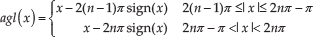
Then, β=agl(β_i−β_j) is the angle from l_i to l_j.

Remark 2. In the remainder of this paper, A₁A₂ denotes the line segment with end-points A₁ and A₂; RL(A₁, A₂) denotes the ray starting from A₁ and passing through A₂; β (A₁, A₂) denotes the direction angle of RL(A₁, A₂); λ_a is a constant such that 0.5< λ_a<1; δ_θ is a small positive constant; and D_S is a positive constant associated with the robots' safety.

3. The Two-direction Path Algorithm

For assigning each robot a reasonable task-point, the host robot should obtain the optimal paths from R_i (i=1, 2,…, m) to all task-points first of all. A two-direction path algorithm is presented in this section for the problem, which is inspired by the fact that the host robot knows the shape of the object beforehand and that all the task-points are around and close to the object.

For the convenience of introducing the method, some important notations are given.

• 1.

  V: a set consisting of all the task-points and all the end-points of the segments on the boundary of the object. Furthermore, all the points in V are continuously numbered in the order encountered by a light-spot such that it starts from a point A on the boundary of the object and moves forward along the boundary of the object continuously until reaching A again.

Remark 3. In this paper, if the light-spot is very close to a point in V, then it is said that the light-spot encounters that point.

For example, In Fig. 1, V={V₁, V₂,…, V₄₂}, where V₁ and V₄₂ are the first and last points encountered by the light-spot respectively.

• 2.

  [o_ij]: an n × n matrix calculated using the following method, where n is the number of points in V.

If i=j, then o_ij=0. Else, if V_iV_j is blocked by the object (V_iV_j has such points that they are on the object but not on the boundary of the object), then o_ij is a positive constant with a very large value. Else, o_ij is the length of V_iV_j.

For example, in Fig. 1, V₁V₅ is blocked by the object, so o₁₅ is very large; V₁V₄ and V₁V₂ are not blocked by the object, so o₁₄ and o₁₂ are the lengths of V₁V₄ and V₁V₂ respectively.

• 3.

  opath: an array about the optimal paths and their lengths from each robot to each point in V, where opath{i}{j} is the record about the optimal path from R_i to V_j.

• 4.

  todo: an increasing permutation of the index numbers of the points in V, where only when the optimal path from V_j1 to R_i has been obtained can j1 be an element in todo. Moreover, if the first element in todo is j, then the last element in todo is j+n, and the index number of V_j1 should be changed to j1+n when j1< j, which implies that V_j1+n is the same point as V_j1. As such, the first and last elements in todo are the points in V with the smallest and largest index numbers, respectively, although they are a same point.

Figure 1.

An illustration of the set V

At the initial stage, todo is obtained using the following method: 1) for each l such that P_RiV_l is not blocked by the object, l is an element of the increasing permutation todo; 2) let the last element in todo be j+n, where j is the first element in todo.

For example, for R₁ in Fig. 1, todo is {7, 8, 9, 10, 23, 38, 39, 40, 49} at the initial stage.

Definition 2. In the case where V_lV_j1 is not blocked by the object and j1 is an element in todo, 1) if j1>l and V_lV_j2 is blocked by the object for any element j2 that is in todo and larger than j1, then the combination of V_j1's optimal path to R_i and V_j1V_l is the positive direction path of V_l to R_i; 2) if j1<l and V_lV_j2 is blocked by the object for any element j2 that is in todo and less than j1, then the combination of V_j1's optimal path to R_i and V_j1V_l is the negative direction path of V_l to R_i.

Based on Definition 2, Theorem 1 can be stated, which is the foundation of the two-direction path algorithm and the reason for the name of the method.

Theorem 1. For a point V_l in V such that the optimal path from V_l to R_i has not been calculated, if both the positive direction and negative direction paths of V_l to R_i have been obtained, then the shorter one of the two paths is the optimal path of V_l to R_i, namely, the shortest path from V_l to R_i that is not blocked by the object.

Proof. Without loss of generality, assume that the optimal path of V_l to R_i is the polyline V_lV_j1V_j2…P_Ri, and j1>l, where no three consecutive points of V_l, V_j1, V_j2,…, and P_Ri are on a same straight line. From the assumption above, it follows that V_j1V_j2…P_Ri is the optimal path of V_j1 to R_i.

Assume an element h exists in todo such that h>j1 and V_lV_h is not blocked by the object. As such, V_lV_j1V_j2…P_Ri must intersect with V_lV_h. Without loss of generality, assume that V_j1V_j2 and V_lV_h intersect at point E, as shown in Fig. 2(b). It follows that V_lEV_j2…P_Ri is such a polyline that is not blocked by the object. On the other hand, because V_j1 is not on V_lV_h, the polyline V_lV_j1E is longer than V_lE. As a result, V_lV_j1V_j2…P_Ri is longer than V_lEV_j2…P_Ri, which contradicts the condition that V_lV_j1V_j2…P_Ri is the optimal path of V_l to R_i.

Figure 2.

Two solutions for the same linear assignment problem. (a) T₁ to R₂, T₂ to R₃ and T₃ to R₃ (b) T₁ to R₃, T₂ to R₂ and T₃ to R₃.

Thus, there is no element h existing in todo such that h>j1 and V_lV_h is not blocked by the object. The conclusion implies that if the polyline V_lV_j1V_j2…P_Ri is the optimal path of V_l to R_i and j1>l, then the polyline is V_l's positive direction path to R_i.

Similarly, it can be proven that if the polyline V_lV_j1V_j2…P_Ri is the optimal path of V_l to R_i and j1<l, then it is V_l's negative direction path to R_i. □

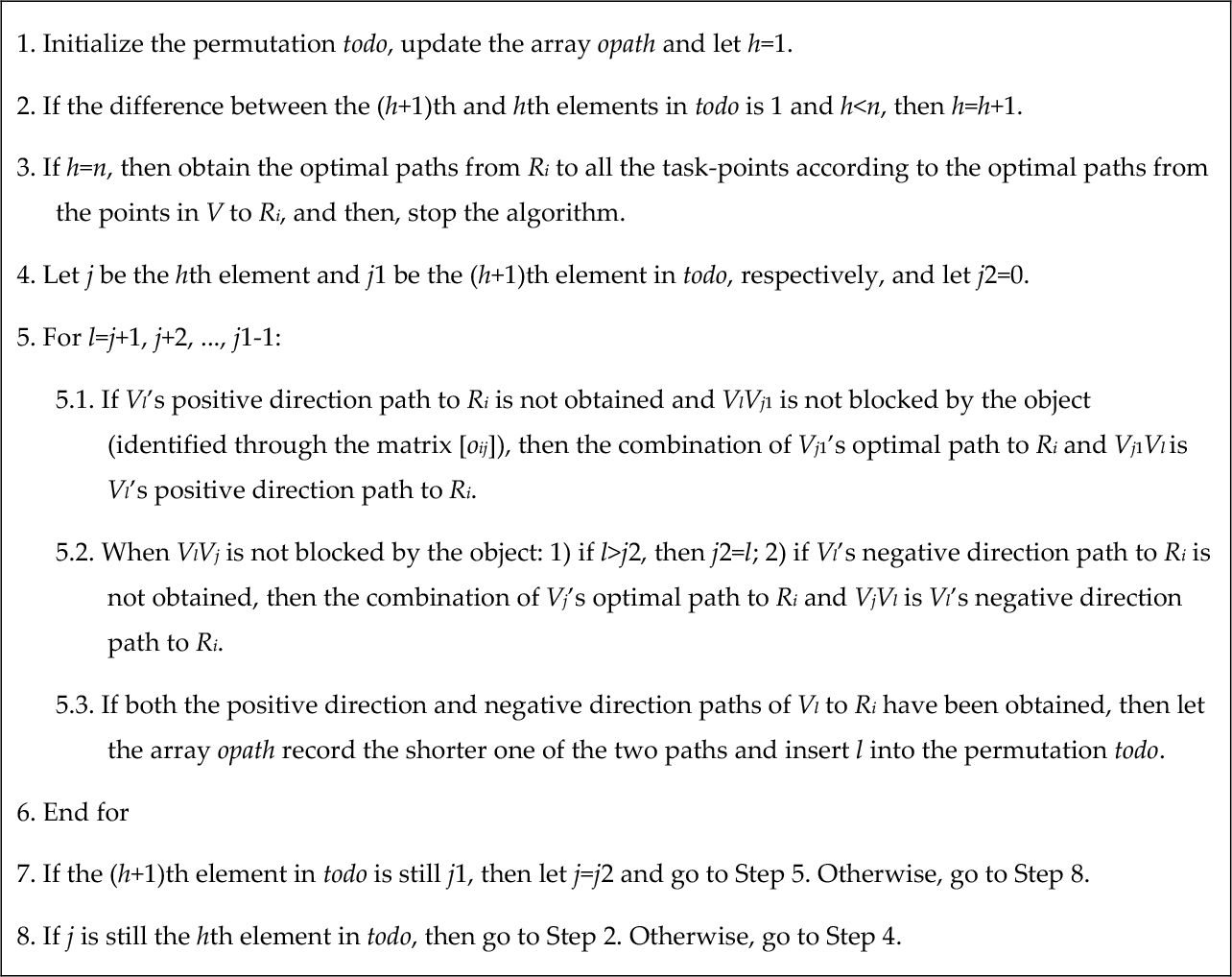
Based on Theorem 1, the two-direction path algorithm is given in Algorithm 1.

From Algorithm 1, it can be seen that the two-direction path algorithm is an improvement of Dijkstra's algorithm since the set todo in the two-direction path algorithm is equivalent to the set of the settled nodes in Dijkstra's algorithm [17] and both of them operate in phases.

Algorithm 1.

Two-direction path algorithm for the optimal paths from R_i to all task-points

1. Initialize the permutation todo, update the array opath and let h=1. 2. If the difference between the (h+1)th and hth elements in todo is 1 and h<n, then h=h+1. 3. If h=n, then obtain the optimal paths from R_i to all the task-points according to the optimal paths from the points in V to R_i, and then, stop the algorithm. 4. Let j be the hth element and j1 be the (h+1)th element in todo, respectively, and let j2=0. 5. For l=j+1, j+2, …, j1-1: 5.1. If V_l's positive direction path to R_i is not obtained and V_lV_j1 is not blocked by the object (identified through the matrix [o_ij]), then the combination of V_j1's optimal path to R_i and V_j1V_l is V_l's positive direction path to R_i. 5.2. When V_lV_j is not blocked by the object: 1) if l>j2, then j2=l; 2) if V_l's negative direction path to R_i is not obtained, then the combination of V_j's optimal path to R_i and V_jV_l is V_l's negative direction path to R_i. 5.3. If both the positive direction and negative direction paths of V_l to R_i have been obtained, then let the array opath record the shorter one of the two paths and insert l into the permutation todo. 6. End for 7. If the (h+1)th element in todo is still j1, then let j=j2 and go to Step 5. Otherwise, go to Step 8. 8. If j is still the hth element in todo, then go to Step 2. Otherwise, go to Step 4. Algorithm 2.

Method for the bottleneck-linear assignment problem

1. According to the PCM, a solution y for the general linear assignment problem is computed by a method such as the shortest augmenting path algorithm [18, 22]. 2. The largest element d_i1j1 in y is selected. 3. If there is an element d_i2j2 in y such that |di1j1+di2j2-di1j2-di2j1|<δ_θ and max (d_i1j2, d_i2j1)< max (d_i1j1, d_i2j2), then d_i1j2 and d_i2j1 are substituted for d_i1j1 and d_i2j2, and then return to Step 2. Otherwise, stop the algorithm.

However, at each phase, all the unsettled nodes need to be considered and only the node with the smallest tentative distance can become settled in Dijkstra's algorithm [17]. In the two-direction path algorithm, however, only the index numbers between j and j1 need to be considered, and two or even more of them can be added to todo (but not always just one).

For example, for R₁ in Fig. 1, four index numbers, namely 11, 12, 13 and 14, are added to todo in the phase such that j=10 and j1=23.

Additionally, the two-direction path algorithm can always compute the optimal paths from R_i to all the task-points.

Because of the advantages mentioned above, the two-direction path algorithm is more efficient than Dijkstra's algorithm for the problem discussed in this section.

4. Bottleneck-linear Assignment

Once the optimal paths from R_i(i=1, 2,…, m) to all the task-points are calculated, a matrix shown as (2) can be obtained, where d_ij(i, j=1, 2,…, m) is the length of the optimal path from a robot R_i to a task-point T_j. The matrix is called the “path cost matrix” (PCM).

$PCM=\left[\begin{array}{cccc}{d}_{11}& d_{12}& \cdots & d_{1m}\\ d_{21}& d_{22}& \cdots & d_{2m}\\ ⋮& ⋮& \ddots & ⋮\\ d_{m1}& d_{m2}& \cdots & d_{mm}\end{array}\right]$

(2)

The problem of assigning to each robot a different task-point is reduced to selecting m elements from the PCM such that no two selected elements are on a same row/column, and if d_ij is selected, then T_j is assigned to R_i.

For optimizing the paths travelled by the robots, it is a good idea to reduce the above problem to a linear assignment problem [18, 22]. The reason for this is that the assignment can set the sum of the selected elements as a minimum. Many methods [18, 22] can be used to solve the assignment problem, and the shortest augmenting path algorithm is one of the best methods for this problem thus far [18].

However, linear assignments focus only on the sum but not on the maximum element of the selected elements. As such, the time taken by the last robot to reach its task-point or used to establish a transportation formation may be quite long. The reason for this is that several solutions exist for the same linear assignment problem in general, and the difference between their largest elements is often great.

For example, in Fig. 2, if the linear assignment is used to assign the task-points to the robots, then two solutions shown as Fig. 2 exist. Obviously, the time taken by the last robot to reach its task-point in Fig. 2(b) will be longer than that in Fig. 2(a) if the conditions are the same as each other.

If bottleneck assignment [18] is used to select m elements from the PCM, then the time taken to establish formations can be optimized as it can make the maximum element of the selected elements a minimum. Yet the assignment ignores the sum of the selected elements. This is to say, except for the path of the last robot to reach its task-point, the travelling paths of all the other robots are ignored. Thus, bottleneck assignment is not suitable either.

From the previous discussion, it follows that a better assignment would be to inherit the advantages of the bottleneck and linear assignments while overcoming their shortcomings. The bottleneck-linear assignment defined below is just an assignment as noted above.

Definition 3. For m elements selected from the PCM such that no two of them are in the same row/column and their sum is a minimum, if their largest element is not larger than the largest one of any other m elements in the PCM such that no two of them are in the same row/column and their sum is a minimum, then the assignment determined by the m selected elements is a bottleneck-linear assignment.

The method for the bottleneck-linear assignment problem is given in Algorithm 2.

Bottleneck-linear assignment has many advantages. For example, compared with general linear assignments, it can make the time taken to form a transport formation as short as possible; compared with general bottleneck assignments, it can optimize the paths travelled by all the robots and not just the last robot.

In fact, the features of bottleneck-linear assignment are closest to those of distance-optimization correspondence as proposed in [23]. But for a distance-optimization correspondence, only the elimination method developed in [23] has been used so far. Under the method, the maximum un-eliminated element in the PCM is picked first of all. If the elimination of the element will entail that no m elements can be selected such that no two of them are in the same row/column, then the element is selected. Otherwise, the element is eliminated. The above steps are repeated until m elements are selected. The difficulty of the elimination method is to determine whether an element can be eliminated - a large amount of calculation is needed to do so in general. Thus, distance-optimization correspondence is more difficult to solve than bottleneck-linear assignment.

5. Improved Artificial Moment Motion Controller

Once each robot has a different task-point, a decentralized motion controller can be used to drive each robot safely and independently towards its task-point.

This paper adopts the artificial moment motion controller developed in [19, 20] because it has many advantages. For example, the controller can make a robot reach a target position with obstacles nearby while having a given posture, and it can make robots pass through narrow passages and bypass complicated obstacles safely, as well as resolving the conflicts between robots quickly while avoiding deadlock and livelock situations even in crowded dynamical environments.

The basic idea of the controller is that, at a given time t_k, R_i may be influenced by three types of artificial moments, namely, the attractive moment by its attractive-point P_ati and attractive angle θ_ati, repulsive moments by obstacles, and coordinated moments by other robots. Under the influence of the artificial moments, R_i changes its PMDline and position along the gradient of the total moments so that the moments can increase quickly. Together with a motion vector (S_xi(k+1), S_yi(k+1)) ^T , which is along R_i's PMDline in general and which is not influenced by the artificial moments, R_i moves one step to the next position. At the next sampling time, the above process is repeated until the task of the system is fulfilled.

From the basic idea of the controller, it can be observed that the attractive point P_ati should be obtained first of all. A feasible method for P_ati is that based on attractive segments [20, 21], which is believed to be better than that in [19]. The reason for this is that since each attractive segment can be used for several sampling times in general, and can be updated in a timely fashion when necessary, attractive segments can decrease the computational burden for attractive points while guiding R_i to move along a suboptimal path.

However, the method given in [21] for computing new attractive segments involves a heavy computational burden while difficult to understand.

For the above limitations, an improved method for attractive segments is presented in this paper. The method is motivated by the fact that the optimal path from R_i to its task-point T_j, which must be a polyline with vertexes in V, is computed by the host robot.

Let A_stiA_endi denote the attractive segment of R_i at time t_k and A_sti(k−1) A_endi(k−1) denote this at t_k-1, where A_sti is on the object and A_endi is in free space in general.

Assume that the optimal path from R_i to its task-point T_j is the polyline V_j0V_j1V_j2…V_jqT_j, where V_j0 is P_Ri. Obviously, if P_RiT_j is not blocked by the object, then q=0.

Let V_jp denote A_sti(k−1). As such, the basic idea for A_sti and A_endi can be introduced as follows.

Because an attractive segment can be employed for several sampling times, A_sti is A_sti(k−1) or V_jp in general. If A_sti cannot be V_jp, then A_sti is V_j(p+1) in the case where p<q and is empty in the case where p=q. The reason for this is that if A_sti cannot be V_jp and p=q, then T_j can be selected as P_ati directly.

A_endi is computed based on A_sti under the following method. If A_sti is empty, then A_endi is empty as well. Otherwise, A_endi is a point such that agl(β(A_sti, A_endi)-β(P_Ri, A_sti))=sgn*θ_a, and the length of A_stiA_endi is λ_aDs, where sgn =sign(agl(β(V_j(p-1), V_jp)-β(V_jp, V_j(p+1)))). The method for θ_a is as follows. If |agl(β(A_sti, V_j(p+1)))-β(A_sti, P_Ri))|>π/2, then θ_a =π/2, else θ_a =|agl(β(A_sti, V_j(p+1)))-β(A_sti, P_Ri))| +δ_θ, where if p=q, then V_j(p+1) is T_j.

The details of the method for A_sti, A_endi and P_ati are given in Algorithm 3, where if t_k=t₀, then p=0; if q>0, then A_sti(−1) and A_endi(−1) are V_j1 and P_Ri, respectively, else they are empty.

If A_sti and A_endi cannot be the same as that at t_k-1 and the method presented in [21] is used to compute them, then the general steps are as below. First, positive and negative key obstacle function segment sets are computed according to the key block wall of R_i. Second, a reasonable motion direction is selected based on the key obstacle function segment sets and R_i's task-point. Finally, A_sti and A_endi are calculated.

Compared with the method in [21], it follows that Algorithm 3 decreases the computational burden for attractive segments for the obvious reasons that Algorithm 3 has no requirement to compute R_i's key block wall, its key obstacle function segment sets or its motion direction, and so forth.

Based on P_ati, the attractive angle θ_ati, which is β(P_Ri, P_ati) in most cases, can be obtained by the method presented in [20]. Unlike that in [20], P_ati needs no improvement in the process for computing θ_ati in this paper. The reason for this is that, because T_j is always close to the object, R_i cannot block the other robots' paths to their task-points when R_i is on T_j.

Algorithm 3.

Compute A_sti, A_endi and P_ati at time t_k

1. If p>q, then P_ati=T_j, and both A_sti and A_endi are empty, and then stop the algorithm. 2. If the distance from P_Ri to RL(A_sti(k-1), A_endi(k-1)) is larger than S_R, then A_sti=A_sti(k-1) and A_endi= A_endi(k-1), and go to Step 6. Otherwise, go to Step 3. 3. If P_RiV_j(p+1) is not blocked by the object, then p=p+1, and go to Step 4. Otherwise, go to Step 5. 4. If p>q, then P_ati=Tj, and both A_sti and A_endi are empty, and then stop the algorithm. Otherwise, go to Step 5. 5. A_sti=V_jp; A_endi is a point such that agl(β(A_sti, A_endi)-β(P_Ri, A_sti))=sgn*θa, and the length of A_stiA_endi is λaDs, where sgn=sign(agl(β(V_j(p-1), V_jp)-β(V_jp, V_j(p+1)))). θa is calculated using the following methods. If |agl(β(A_sti, V_j(p+1)))-β(A_sti, P_Ri))|>π/2, then θa =π/2, else θa =|agl(β(A_sti, V_j(p+1)))-β(A_sti, P_Ri))| +δθ. 6. Let P_ati=A_endi, and then stop the algorithm.

The artificial motion controller designed in [20] can be used to make R_i move towards and reach T_j.

In the controller, except for some special cases, the length of the motion vector (S_xi(k+1), S_yi(k+1)) ^T is S_R. As such, R_i's motion speed will be high in most cases, even though the sum of the artificial moments imposed on R_i is zero. Thus, it is difficult for R_i to become trapped by obstacles and it can pass through narrow passages.

In general, the attractive moment by P_ati and θ_ati will make R_i’s PMDline point to P_ati (i.e., it will make the direction angle of R_i’s PMDline be θ_ati) and the repulsive moments by obstacles will keep R_i’s PMDline away from obstacles. Because of the motion vector (S_xi(k+1), S_yi(k+1)) ^T , R_i can move close to P_ati while staying away from obstacles.

If another robot R_j is close to R_i, then R_j may impose a coordinated moment on R_i so that the conflicts between them can be resolved safely and quickly. The moment is designed according to the following idea. If they have no tendency to move towards each other, then R_j's coordinated moment will only make R_i maintain a safe distance from R_j. Otherwise, the coordinated moment will make R_i move to one side of R_j so that R_i can bypass R_j and so that no collision occurs between them.

For the artificial moment motion controller and the various concepts that are not specified in this paper, readers may refer to [20] for details since they are the same as those in [20].

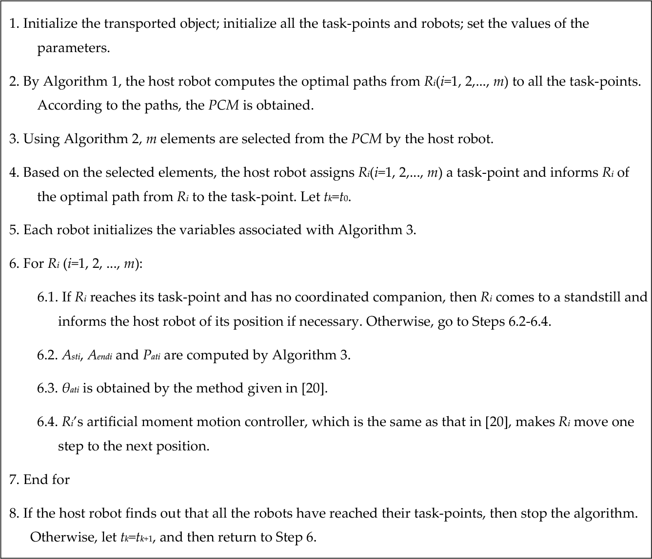
The details of the proposed method for forming complex transport formations are given in Algorithm 4.

6. Simulations and Analysis

For verifying the feasibility and efficiency of the proposed method, extensive simulations have been carried out. The results of three typical simulations are given in Figs. 3–5, where all the algorithms are written in the MATLAB language. Some parameters are that D_S=1.2, λ_a=0.8, δ_θ=π/90, D_R=0.15 and S_R=0.24.

Figure 3.

Simulation for 23 robots to form a complex transport formation

Figure 4.

Simulation for 32 robots to form a complex transport formation

Figure 5.

Simulation for 43 robots to form a complex transport formation

As a comparison, the simulations based on general linear assignment are also given with the same parameters and conditions.

In the simulations, the task-points of each robot determined by general linear assignment and bottleneck-linear assignment are shown in Tabs. 1–3, where “R” denotes the indexes of the robots and “GL” and “BT” denote the task-points of the robots determined, respectively, by general linear assignment and bottleneck-linear assignment.

Table 1.

Assignment results of the task-points in the simulation with 23 robots

R	1	2	3	4	5	6	7	8	9	10	11	12	13	14	15	16	17	18	19	20	21	22	23
GL	14	7	21	8	16	10	22	12	17	5	18	4	1	15	20	3	6	11	19	9	2	13	23
BT	14	7	21	2	16	10	22	12	17	5	18	8	23	15	20	9	6	11	19	3	1	13	4

Table 2.

Assignment results of the task-points in the simulation with 32 robots

R	1	2	3	4	5	6	7	8	9	10	11	12	13	14	15	16	17	18	19	20	21	22	23	24	25	26	27	28	29	30	31	32
GL	29	20	24	27	21	19	31	1	2	4	5	15	6	17	16	13	12	10	11	8	22	26	32	23	3	28	9	18	30	7	25	14
BT	21	26	19	27	28	29	31	1	2	4	6	12	8	9	11	17	16	13	15	18	24	22	32	20	3	23	10	5	30	7	25	14

Table 3.

Assignment results of the task-points in the simulation with 43 robots

R	1	2	3	4	5	6	7	8	9	10	11	12	13	14	15	16	17	18	19	20	21	22	23	24	25	26	27	28	29	30	31	32	33	34	35	36	37	38	39	40	41	42	43
GL	7	11	6	12	13	14	15	16	17	19	22	18	24	26	23	27	28	29	30	31	37	38	33	34	32	35	40	41	1	2	3	4	5	8	9	25	10	42	20	36	43	39	21
BT	9	11	7	12	13	14	15	16	17	19	22	18	21	26	23	27	28	29	31	32	33	39	34	35	36	37	40	41	1	2	3	4	5	8	6	25	10	42	24	30	43	38	20

In Figs. 3–5, small circles with PMDlines indicate task-points and those without PMDlines indicate the initial positions of the robots, where the numbers beside them are their indexes. The larger circles with PMDlines are robots, where the solid colour curves are their travelling paths.

From Figs. 3–5, it follows that all the given transport formations are achieved safely and exactly by the proposed method, although the formations are very complex. Furthermore, each robot's PMDline direction can be the same as that of its task-point when the robot reaches its task-point and comes to a standstill. Thus, the proposed method is feasible.

From the robots' travelling paths, it can be seen that most of the robots do not move along the optimal paths to their task-points. The reason for this is that when an optimal path associated with a robot is computed by the host robot, the robot's size, and conflicts with other robots and collisions with the object are not considered for decreasing the computational burden. However, within the process of movement, all the matters mentioned above are required to be considered. As a result, most of the robots cannot move along optimal paths.

Even so, the differences between the robots' travelling paths and the optimal ones are all very slight. Thus, the simulations verify that the method proposed in this paper for attractive segments can not only decrease the computational burden but can also optimize the robots' travelling paths.

Algorithm 4.

General steps for forming a complex transport formation

1. Initialize the transported object; initialize all the task-points and robots; set the values of the parameters. 2. By Algorithm 1 , the host robot computes the optimal paths from R_i(i=1, 2,…, m) to all the task-points. According to the paths, the PCM is obtained. 3. Using Algorithm 2 , m elements are selected from the PCM by the host robot. 4. Based on the selected elements, the host robot assigns R_i(i=1, 2,…, m) a task-point and informs R_i of the optimal path from R_i to the task-point. Let tk=t0. 5. Each robot initializes the variables associated with Algorithm 3 . 6. For R_i (i=1, 2, …, m): 6.1. If R_i reaches its task-point and has no coordinated companion, then R_i comes to a standstill and informs the host robot of its position if necessary. Otherwise, go to Steps 6.2–6.4. 6.2. A_sti, A_endi and P_ati are computed by Algorithm 3 . 6.3. θ_ati is obtained by the method given in [20]. 6.4. R_i's artificial moment motion controller, which is the same as that in [20], makes R_i move one step to the next position. 7. End for 8. If the host robot finds out that all the robots have reached their task-points, then stop the algorithm. Otherwise, let t_k=t_k+1, and then return to Step 6.

In the figures (b) and (d), the time elapsed or steps used to form the provided formations are given. From the results, it follows that the time elapsed or steps used based on bottleneck-linear assignment are much lower than those based on general linear assignment. The result indicates that bottleneck-linear assignment is highly beneficial for the problem discussed in this paper.

7. Conclusions

This paper proposes a method based on bottleneck-linear assignments for assigning each robot a reasonable task-point. An improved artificial moment motion controller is used to make each robot move safely towards its task-point while its travelling path is shorter. The following aspects of this paper deserve further attention.

1. The two-direction path algorithm. The algorithm is the foundation of the task-points' assignment as it can compute the optimal paths from R_i (i=1, 2,…, m) to all the task-points. Although some aspects of the algorithm are similar to those of Dijkstra's algorithm, it has many advantages. For example, the algorithm can always compute the optimal paths from R_i to all the task-points; at each stage, only some of the elements' index numbers that are not in todo are considered, and the number of the elements in todo may increase by two or more (but not always by one). Thus, the algorithm is more efficient than Dijkstra's algorithm.

2. The bottleneck-linear assignment and the method for the assignment. The assignment has many advantages. For example, compared with general linear assignments, it can make the time used to form a transport formation become as short as possible; compared with general bottleneck assignments, it can optimize the travelling paths of all the robots and not just the last robot; compared with the distance-optimization correspondence, it is easier to solve.

3. The improved method for attractive segments. The method is based on the fact that the optimal path of R_i to its task-point has been computed by the host robot at the initial stage. Moreover, if necessary, a new attractive segment for R_i can be quickly calculated by the method while there is no requirement to compute R_i's key block wall, key obstacle function segment sets or motion direction, and so forth. Thus, the method decreases the computational burden for attractive segments considerably, and the performance of the artificial moment motion controller is improved when it is implemented in real-time.

In the future, we will investigate how to use the strategy based on the artificial moments to control complex multi-robot transport formations so that the transported objects can be moved to desired positions.