Modelling of Airship Flight Mechanics by the Projection Equivalent Method

Abstract

This article describes the projection equivalent method (PEM) as a specific and relatively simple approach for the modelling of aircraft dynamics. By the PEM it is possible to obtain a mathematic al model of the aerodynamic forces and momentums acting on different kinds of aircraft during flight. For the PEM, it is a characteristic of it that -in principle - it provides an acceptable regression model of aerodynamic forces and momentums which exhibits reasonable and plausible behaviour from a dynamics viewpoint. The principle of this method is based on applying Newton's mechanics, which are then combined with a specific form of the finite element method to cover additional effects. The main advantage of the PEM is that it is not necessary to carry out measurements in a wind tunnel for the identification of the model's parameters. The plausible dynamical behaviour of the model can be achieved by specific correction parameters, which can be determined on the basis of experimental data obtained during the flight of the aircraft. In this article, we present the PEM as applied to an airship as well as a comparison of the data calculated by the PEM and experimental flight data.

1. Introduction

One of the first methods solving the problem of calculating airship aerodynamics is the so-called “thin body theory” [1–3]. Expanding and extending this theory of influencing factors like the wind impact [4] and the viscous forces impact [5] provides more complex solutions to this problem. Some works which solve the aerodynamics of airship flight analytically are given in [6–9]. In principle, all actual analytical methods are based on the complex approach of the thin body theory with Munk's correction factors. In reality, the aerodynamics problem is very complex and its solution is dependent on a variety of parameters. It is well known that if the body's geometrical structure is more complex, then “parasitic effects” will exist which act on the body. These effects can be derived from airflow aerodynamics. Such effects (flow separation, streamlines curving) cause smaller or larger deviations between reality and the corresponding analytical model. Due to these reasons computational fluid dynamics (CFD) methods [10, 11] have been derived for the calculation of aerodynamic forces. CFD methods use measured data from wind tunnels for modelling. Using CFD methods it is possible to create advanced models which can consider specific parasitic effects. CFD methods are particularly advanced, but they require laboratory experimental equipment to be set up and a lot of computing time for calculations. This means that detailed research into aerodynamics requires tremendous efforts and many resources. Nowadays, this research can be realized only in highly specialized companies or research institutes.

However, in such cases where it is necessary to design a control system for already existing flying machines which are already optimized from constructional aspects, it is still important to create a specific regression model of a system's flight mechanics which is sufficient for the design of any on-board control systems. The key role of this specific regression model is to provide a plausible mathematical description of a system's dynamic flight behaviour.

In this article, we present a specific method that allows for the creation of this mathematical regression model so that its structure and extent are not too complicated for online calculation with the typical light-weight computer hardware of a small airship. This method provides a dynamic model with specific correction parameters which can be easily identified on the basis of measured data from experimental flights (e.g., without wind tunnel measurement). The regression model of the flight mechanics is derived according to the proposed PEM, which is specifically derived to solve the aerodynamics part of the flight mechanics. The principle of our PEM is based on a suitable decomposition of the flight system into such components, which can be considered as relatively homogeneous from the aerodynamics viewpoint. In the next step, the partial balances of the aerodynamic forces and momentums of each component are calculated separately.

The total aerodynamic forces and momentums acting on the flight system (e.g., an airship) are then given as the sum of these partial aerodynamic forces and momentums. The computation of the partial aerodynamic forces and momentums is carried out by a combination of the standard Newton's mechanics with a specific form of the finite element method with respect to the body's wind side and leeward side.

The PEM's main advantage is that it offers a regression model which for normal flight conditions provides a plausible approximate dynamic description of the system's flight behaviour. All the parasitic or disturbance effects which occur under normal flight conditions are reflected in specific correction parameters.

This article describes the application of our PEM for a small airship (nine metres in length). It shows simulation results which were obtained using a mathematical regression model and it also presents a comparison with airship experimental flight data. More information can be found in [12].

This paper is structured as follows: in Chapter 2, the basic principles of the PEM are shown. In accordance with those PEM principles, Chapter 3 explains the airships decomposition into specific parts. Chapter 4 presents the characteristic parameters of these decomposed parts of the flight system with respect of the wind side and the leeward side of the body parts. Chapter 5 draws conclusions from the previous chapters and it derives the principles for aerodynamic force balance. The resulting balance of the aerodynamic forces and momentums for airship parts, along with a short preview of the complete mathematical model of the airship's flight mechanics, is presented in Chapter 6. In Chapter 7, the list of the model parameters for our experimental airship can be found. Chapter 8 focuses on comparisons with experimental flights of a real airship. The conclusion and discussion of the PEM are given in Chapter 9. A literature list can be found at the end of this paper.

2. The PEM principle

The principle of the PEM can be described by the following steps:

1. Suitable airship decomposition into the specific parts: the airship is divided into parts which can be considered as relatively homogeneous from an aerodynamics viewpoint.

2. For all the specified parts, the following parameters have to be determined: projection surface areas and their geometrical centres with respect to the airship's body frame (coordination system), translational velocities for all the geometrical centres of the projection surfaces, and the wind velocity, which is expressed separately for every projection surface with respect to its body frame.

3. For specific airship parts which include the centre of rotation (in this case, the hull) it is necessary to apply a specific form of the finite element method, as described in the next section of this article where it is called the “single cuts” method.

4. Using Newton's mechanics, the aerodynamic force balances for every projection surface of the airship's parts can be realized with respect to the wind side and the leeward side.

5. The computed aerodynamic forces are then transformed from the projection surfaces frame to the airship body frame.

6. Considering the position vectors to all the projection surfaces (their geometrical centres) and their related aerodynamic force values, which are expressed in the airship body frame, all the forces and momentums can be determined with respect to the airship's centre of rotation.

The total aerodynamic forces and momentums acting on the airship are then given as the sum of all these partial aerodynamic forces and momentums.

3. Airship decomposition to the specific parts

During some research projects in flight robotics, the Control Systems Engineering group of the FernUniversität in Hagen acquired a small airship (length 8.7 m, diameter 2.38 m, volume 24 m³) for experimental purposes. This airship is presented in “Fig. 1”.

Figure 1.

Airship body frame (coordination system NED) and specific components (1 – hull, 2 – rudder fixed body, 3 – rudder flap, 4a – left elevator fixed body, 5a – left elevator flap)

As mentioned earlier, it is necessary to divide the airship into relatively homogeneous components (from an aerodynamics viewpoint) as stressed in “Fig. 1”. On this basis the airship has been divided into: the airship hull, the rudder fixed body (without a flap) and the rudder flap (without the fixed body), the left elevator fixed body and the left elevator flap, and the right elevator fixed body and the right elevator flap.

4. Characteristic parameters of the airship parts

Based on photos of the airship, a computer model of our flight system was created (i.e., with “SolidWorks”). From this model, all the following parameters were determined: position vectors of the CV (centre of volume), the CG (centre of gravity) location, the projection surface areas and their geometrical centres with respect to the airship body frame, the translational velocities for all the geometrical centres of the projection surfaces, and the wind velocity, which is expressed separately for every projection surface with respect to its body frame. The airship hull includes the centre of rotation CR (CR ≡ CV). For this component, it is necessary to apply the specific method of “single cuts”, which is described in a separate chapter of this article. Before any specific parameters are determined for the airship components, it is necessary to define the airship's translational velocity V, the wind velocity W and the airship angular velocity Ω with respect to the airship body frame,

$\begin{array}{l}V={\left(\begin{array}{ccc}{v}_{\mathrm{x}}& v_{\mathrm{y}}& v_{\mathrm{z}}\end{array}\right)}^{\mathrm{T}},W={\left(\begin{array}{ccc}{w}_{\mathrm{x}}& w_{\mathrm{y}}& w_{\mathrm{z}}\end{array}\right)}^{\mathrm{T}},\\ \mathrm{\Omega }={\left(\begin{array}{ccc}{\omega }_{\mathrm{x}}& {\omega }_{\mathrm{y}}& {\omega }_{\mathrm{z}}\end{array}\right)}^{\mathrm{T}}\end{array}$

(1)

a. Rudder's parameters

The rudder is divided into its fixed body and a flap part, as shown in “Fig. 2”. The fixed rudder body is balanced with respect to the airship's body frame. Because the connected rudder flap can be rotated, a separate body frame can be defined for the rudder flap, which is nominated and labelled as the “K-frame” here.

Figure 2.

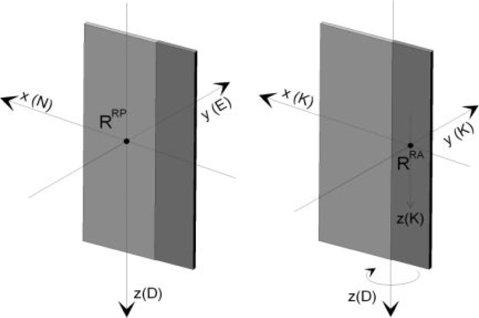
The fixed rudder body (left) and the rudder flap with its body frame K (right)

For the fixed rudder body, we define the projection surface S_y^RP of the fixed rudder body which is orthogonal in the y-axis direction, the position vector R ^RP for the geometric centre of the surface S_y^RP and the translational velocity V ^RP = (V + Ω x R ^RP) for the geometric centre R ^RP.

For the rudder flap, we define the projection surface S_y^RA(K) of the rudder flap which is orthogonal to the y(K) -axis direction, the position vector R ^RA for geometric centre of the surface S_y^RA(K), the rudder flap angle ɛ, the translational velocity V ^RA(K) = f((V + Ω x R ^RA), ɛ) for the geometric centre R ^RA, and the wind velocity W (K) = f (W, ɛ) expressed in the rudder flap body frame K. For simplicity, the rudder thickness is neglected and for the position vector R ^RA it is considered that it is independent of the rudder flap angle ɛ.

b. Elevators' parameters

As with the rudder, we proceed as outlined in “Fig. 3”. The only difference is that both elevators can be rotated in the airship's body frame around a constructional angle ±η (the left elevator is rotated about the +η angle and the right elevator about the -η angle). The constructional angle ±η together with the left elevator flap angle μ and the right elevator flap angle è have to be considered for the wind velocity W transformation and the airship translational velocity V transformation, which it is necessary to apply between the body frames defined for the elevators' fixed bodies and the elevators' flaps and airship body frame. For simplicity, the elevator fixed body thickness is neglected. For the constructional angle, it is considered that η⁺ = − η⁻. In the next step, it is considered that the left and right elevator are the same size and so it is sufficient to determine only the following parameters.

Figure 3.

The fixed body frames E⁺ and E⁻ of the left and right elevators (left figure), and the flap body frames E⁺_μ and E⁻_σ of the left and right elevators (right figure)

For the fixed body of the left and right elevator, we determine the projection surface S_z^EP(E±) of the left and right elevator fixed bodies (both surfaces are equivalent) which are orthogonal to the z(E^±) -axis direction, the position vectors R ^EP+ and R ^EP- for the geometric centres of the left and right elevator fixed body surfaces S_z^EP(E⁺) and S_z^EP(E⁻), the constructional angle for the left η⁺ and the right η⁻elevators, respectively, the translational velocities V ^EP+(E⁺) = f((V + Ω X R ^EP+), η⁺) and V ^EP-(E⁻) = f((V + Ω x R ^EP-), η⁻) for the geometric centres R ^EP+ and R ^EP-, and the end wind velocities W (E⁺) = f(W, η ⁺ ) and W (E⁻) = f(W, η⁻) expressed in the body frame of the left E⁺ and right E⁻ elevator fixed bodies, respectively.

For the left and right elevator flaps, we determine the projection surface S_Z^EA(E^±_μ|Σ) of the left and right elevator flaps (both surfaces are equivalent) which are orthogonal to the z(E^±_μ|σ)-axis direction, the position vectors R ^EA+ and R ^EA- for the geometric centres of the left and right elevator flap surfaces S_Z^EA(E^+μ) and S_Z^EA(E⁻_Σ), the control angle for the left μ and right σ elevator flaps, the translational velocities V ^EA+(E⁺_μ) = f((V + Ω x R ^EA+), η⁺, μ) and V ^EA-(E⁻_Σ) = f((V + Ω X R ^EA-), η⁻, Σ) for the geometric centres R ^EA+ and R ^EA-, respectively, and the end wind velocities W (E⁺_μ)= f(W, μ) and W (E⁻_Σ) = f(W, Σ) expressed in the body frame of the left E⁺_μ and right E⁻_σ elevator flaps, respectively. For simplicity, it is considered that the position vectors R ^EA+ and R ^EA- are independent of the left and right rudder flap angles μ and σ.

c. Airship hull and the “single cuts” method

The airship hull includes the centre of rotation CR (CR ≡ CV). For this reason, it is necessary to apply the specific single cuts method as one tool of the PEM. First, the airship's hull is split into all three orthogonal planes which are defined in the 3D airship body frame. Every cut surface of the airship's hull is next divided into four quadrants. For every quadrant, specific parameters are determined, which is the topic of this chapter. Any real airship hull can be treated in principle as a deformed ellipsoid. Cuts of this airship hull and their quadrants are illustrated in “Fig. 4”.

Figure 4.

3D orthogonal hull cuts with four quadrants: a) the front view, surface S_x, b) the side view, surface S, and c) the view from above, surface S_z

After cutting the airship hull, three orthogonal surfaces S_x, S_y and S_z can be identified. Each surface is derived from a cut which is an orthogonal projection of the hull body to the relevant axis direction of the airship body frame. This means that S_x is the projection surface which is orthogonal to the x-axis direction, S_y is a projection surface which is orthogonal to the y-axis direction, and S_z is a projection surface which is orthogonal to the z-axis direction. The projection surfaces S_x (the yz plane of the airship body frame), S_y (the xz plane of the airship body frame) and S_z (the xy plane of the airship body frame) are divided into four parts, labelled I, II, III and IV (see “Fig. 4”). These parts of the surfaces S_x, S_y and S_z are also labelled as partial surfaces S_x^I to S_x^IV, S_y^I to S_y^IV and S_z^I to S_z^IV. For these surfaces, we can determine the corresponding sizes, the position vectors R ⁱ _sx, R ⁱ _sy and Rⁱ_sz, and the translational velocities V ⁱ _Sx = V + Ω x R ⁱ _sx, V ⁱ _Sy = V + Ω x R ⁱ _sy and V ⁱ _Sz = V + Ω x R ⁱ _sz for the geometric centres of the partial projection surfaces ∀ i = 1, 2, 3, 4.

d. The wind side and leeward side of the body

As mentioned above, the PEM balances the body wind side and the body leeward side. For this purpose, we first define the surfaces S_i in the body frame such that these surfaces S_i are orthogonal to the direction of one of the three axes of the body frame. Let us define a surface S_y which is orthogonal to the y-axis direction of the body frame, let its translational velocity be assigned as V, and let the wind velocity be assigned as W, such that

$\begin{array}{l}W={\left(\begin{array}{ccc}{w}_{\mathrm{x}}& w_{\mathrm{y}}& w_{\mathrm{z}}\end{array}\right)}^{\mathrm{T}}={\left(\begin{array}{ccc}0& w_{\mathrm{y}}& 0\end{array}\right)}^{\mathrm{T}}\text{and}\\ V={\left(\begin{array}{ccc}{v}_{\mathrm{x}}& v_{\mathrm{y}}& v_{\mathrm{z}}\end{array}\right)}^{\mathrm{T}}={\left(\begin{array}{ccc}0& v_{\mathrm{y}}& 0\end{array}\right)}^{\mathrm{T}}\end{array}$

(2)

In the next step, it is necessary to consider both sides of surface S _y. One side of the surface S_y which is oriented to the positive direction of the y-axis is indicated as S_y+ and the second side of this surface S_y is indicated as S_y-. If the surface S_y is in motion, then the velocities V and W are summed or subtracted depending on the proper combination between the wind direction and the surface movement direction. This sum (or difference) is not equal for the S _y+ side and the S_y- side. This velocity is called the “specific sum velocity” and it is denoted U ^Σ_y+ for the S_y+ side and U ^Σ_y-for the S_y- side. In the following step, the question is posed: How can the calculation of the specific sum velocities U ^Σ_y+ and UU ^Σ_y- be carried out? The interaction between the wind velocity and the airship's body motion is very complex. The PEM solves this problem under the following simplifying assumptions:

1. Assumption of the body's full “shielding”

   This assumption considers that the wind flow is completely interrupted by the airship's body. This means that for the leeward sides of the body the airflow velocity is zero.

2. Assumption of the body's full “transparency”

   This assumption considers that wind flow is not influenced at all by the airship's body. This means that for leeward sides of the body the airflow velocity remains unchanged.

These two simplifying cases do not consider several further facts, namely that:

1. The airship's body - when moving forwards - displaces a certain air volume along the body's surface, where it creates a specific airflow.

2. If the body of the airship is in an external airflow, then the geometry of the streamlines and the airflow's velocity profiles are dependent on the actual body geometry, on the material properties of the body surface, and on the airflow velocity itself.

Accepting both of these simplifying assumptions mentioned above will cause deviations from the real body's behaviour in airflow. These model deviations are later compensated for by correction parameters which are determined on the basis of experimental data. The corresponding procedures will be explained later. Note that the decision about which assumption fits better can only be known on the basis of comparing the simulation results with experimental data. Let us assume that, according to the experimental results, it is better to accept the full “shielding” assumption for the airship's flight conditions.

Accordingly, the specific sum velocities U ^Σ_y+ and U ^Σ_y- can be computed on the basis of the following terms.

In accordance with “Fig. 5”, we can write:

Figure 5.

Mutual impact of the surface velocity v_y and the wind velocity w_y on the S_y surface with respect to the assumption of body full “shielding”

1. If the wind velocity w_y is zero or negative w_y≤0, then

$\begin{array}{cc}{U}_{\mathrm{y}+}^{\sum }={\left(\begin{array}{ccc}\left(w_{\mathrm{x}}-v_{\mathrm{x}}\right)& {\left(w_{\mathrm{y}}-v_{\mathrm{y}}\right)}^{\max =0}& \left(w_{\mathrm{z}}-v_{\mathrm{z}}\right)\end{array}\right)}^{\mathrm{T}}& (a)\\ U_{\mathrm{y}-}^{\sum }={\left(\begin{array}{ccc}\left(w_{\mathrm{x}}-v_{\mathrm{x}}\right)& {\left(-v_{\mathrm{y}}\right)}_{\min =0}& \left(w_{\mathrm{z}}-v_{\mathrm{z}}\right)\end{array}\right)}^{\mathrm{T}}& (b)\end{array}$

(3)

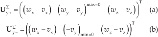
2. If the wind velocity w_y is positive w_y > 0, then

$\begin{array}{cc}{U}_{\mathrm{y}+}^{\sum }={\left(\begin{array}{ccc}\left(w_{\mathrm{x}}-v_{\mathrm{x}}\right)& {\left(-v_{\mathrm{y}}\right)}^{\max =0}& \left(w_{\mathrm{z}}-v_{\mathrm{z}}\right)\end{array}\right)}^{\mathrm{T}}& (a)\\ U_{\mathrm{y}-}^{\sum }={\left(\begin{array}{ccc}\left(w_{\mathrm{x}}-v_{\mathrm{x}}\right)& {\left(w_{\mathrm{y}}-v_{\mathrm{y}}\right)}_{\min =0}& \left(w_{\mathrm{z}}-v_{\mathrm{z}}\right)\end{array}\right)}^{\mathrm{T}}& (b)\end{array}$

(4)

where

${\left(\arg \right)}_{\min =0}=\{\begin{array}{c}\arg \\ 0\end{array}\begin{array}{c}\forall \hspace{0.17em}\text{arg}\in (0,\infty )\\ \forall \hspace{0.17em}\text{arg}\in (-\infty ,0〉\end{array}$

(5)

${\left(\arg \right)}^{\max =0}=\{\begin{array}{c}0\\ \arg \end{array}\begin{array}{c}\forall \hspace{0.17em}\text{arg}\in 〈0,\infty )\\ \forall \hspace{0.17em}\text{arg}\in \left(-\infty ,0\right)\end{array}$

(6)

Equations (3) and (4) respect the assumption that the surface S_y completely impedes any wind flow (“shielding” mode). The leeward side of the surface S_y is represented by S_y+ if the wind direction is identical to the y-axis direction. The leeward side of the surface S_y represent S_y- if the direction of the wind flow is opposite to the y-axis direction. In principle, three body projection planes exist in 3D space. For every projection plane, a surface can be defined which is orthogonal to the x-, y- or z-axis direction. Every projected surface consists of two sides. This means that there are six specific sum velocities U ^Σ which are denoted as U ^Σ_x+, U ^Σ_x- U ^Σ_y+, U ^Σ_y-, U ^Σ_z+, and U ^Σ_z-. These specific sum velocities can be calculated (the assumption of full body “shielding”) according to the following relations:

1. The specific sum velocities U ^Σ_x±(V, W) are given as

$\begin{array}{cc}{U}_{\mathrm{x}+}^{\sum }\left(w_{\mathrm{x}}\le 0\right)={\left(\begin{array}{ccc}{\left(w_{\mathrm{x}}-v_{\mathrm{x}}\right)}^{\max =0}& \left(w_{\mathrm{y}}-v_{\mathrm{y}}\right)& \left(w_{\mathrm{z}}-v_{\mathrm{z}}\right)\end{array}\right)}^{\mathrm{T}}& (a)\\ U_{\mathrm{x}-}^{\sum }\left(w_{\mathrm{x}}\le 0\right)={\left(\begin{array}{ccc}{\left(-v_{\mathrm{x}}\right)}_{\min =0}& \left(w_{\mathrm{y}}-v_{\mathrm{y}}\right)& \left(w_{\mathrm{z}}-v_{\mathrm{z}}\right)\end{array}\right)}^{\mathrm{T}}& (b)\\ U_{\mathrm{x}+}^{\sum }\left(w_{\mathrm{x}}>0\right)={\left(\begin{array}{ccc}{\left(-v_{\mathrm{x}}\right)}^{\max =0}& \left(w_{\mathrm{y}}-v_{\mathrm{y}}\right)& \left(w_{\mathrm{z}}-v_{\mathrm{z}}\right)\end{array}\right)}^{\mathrm{T}}& (c)\\ U_{\mathrm{x}-}^{\sum }\left(w_{\mathrm{x}}>0\right)={\left(\begin{array}{ccc}{\left(w_{\mathrm{x}}-v_{\mathrm{x}}\right)}_{\min =0}& \left(w_{\mathrm{y}}-v_{\mathrm{y}}\right)& \left(w_{\mathrm{z}}-v_{\mathrm{z}}\right)\end{array}\right)}^{\mathrm{T}}& (d)\end{array}$

(7)

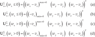
2. The specific sum velocities U ^Σ_z±(V, W) are given as

$\begin{array}{cc}{U}_{\mathrm{z}+}^{\sum }\left(w_{\mathrm{z}}\le 0\right)={\left(\begin{array}{ccc}\left(w_{\mathrm{x}}-v_{\mathrm{x}}\right)& \left(w_{\mathrm{y}}-v_{\mathrm{y}}\right)& {\left(w_{\mathrm{z}}-v_{\mathrm{z}}\right)}^{\max =0}\end{array}\right)}^{\mathrm{T}}& (a)\\ U_{\mathrm{z}-}^{\sum }\left(w_{\mathrm{z}}\le 0\right)={\left(\begin{array}{ccc}\left(w_{\mathrm{x}}-v_{\mathrm{x}}\right)& \left(w_{\mathrm{y}}-v_{\mathrm{y}}\right)& {\left(-v_{\mathrm{z}}\right)}_{\min =0}\end{array}\right)}^{\mathrm{T}}& (b)\\ U_{\mathrm{z}+}^{\sum }\left(w_{\mathrm{z}}>0\right)={\left(\begin{array}{ccc}\left(w_{\mathrm{x}}-v_{\mathrm{x}}\right)& \left(w_{\mathrm{y}}-v_{\mathrm{y}}\right)& {\left(-v_{\mathrm{z}}\right)}^{\max =0}\end{array}\right)}^{\mathrm{T}}& (c)\\ U_{\mathrm{z}-}^{\sum }\left(w_{\mathrm{z}}>0\right)={\left(\begin{array}{ccc}\left(w_{\mathrm{x}}-v_{\mathrm{x}}\right)& \left(w_{\mathrm{y}}-v_{\mathrm{y}}\right)& {\left(w_{\mathrm{z}}-v_{\mathrm{z}}\right)}_{\min =0}\end{array}\right)}^{\mathrm{T}}& (d)\end{array}$

(8)

In other cases, when the assumption of full body “transparency” is appropriate, the following substitutions are valid for equations (3) to (8)

${\left(-v_i\right)}_{\min =0}\leftarrow {\left(w_i-v_i\right)}_{\min =0}\text{and}{\left(-v_i\right)}^{\max =0}\leftarrow {\left(w_i-v_i\right)}^{\max =0}$

(9)

e. The balance of aerodynamic forces

In the PEM we only consider Newton's equation for aerodynamic resistance (drag), which is defined for turbulent flow (although even this relation is of limited relevance only). The lift force, which is usually calculated on the basis of Bernoulli's principle, is not considered here. In the PEM, the “lift” effect is only treated as the result of the Newton's equation applied with specific correction parameters. Newton's equation is defined as

$F=\frac{1}{2}\rho C{S}_{\perp }{v}^2$

(10)

where F is the aerodynamic resistance (drag), ρ is the fluid density (air), C is the resistance coefficient (drag coefficient), S_⊥ is the orthogonal surface to the air streamlines direction, and v is the fluid (air) velocity.

In a further step, we modify Newton's equation (10) towards the PEM form. Let there be a given body frame which is oriented in the same way as the typical frame system NED (north–east–down). All three body projection surfaces S_x, S_y and S_z and a specific sum velocity U^Σ _{i ±} are included in this body frame, as shown in “Fig. 6”.

Figure 6.

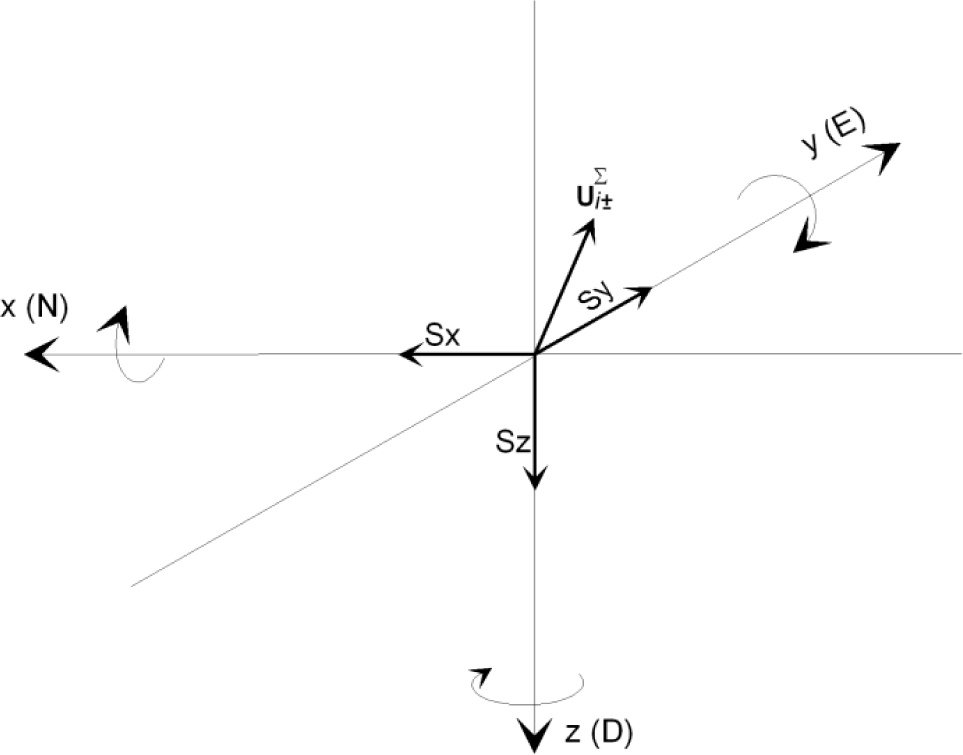
The body projection surfaces and the specific sum velocity

Because equation (10) includes surface S_⊥ which is orthogonal to the direction of the fluid streamlines (in this case, streamlines of air), it is necessary to derive surface S_⊥ from the body projection surfaces S_x, Sy and S_z (which are orthogonal to the axes directions). Therefore, these surfaces have to be projected towards the air flow to substitute them by virtual surfaces which are directly exposed to the wind. These “towards wind” projection surfaces are orthogonal to the specific sum velocity U ^Σ _{i ±}. This means that it is necessary to realize projections of the surfaces S_x, S_y and S_z to the specific sum velocities' directions U ^Σ_x+, U ^Σ_x-, U ^Σ_y+, U ^Σ_y+, U ^Σ_z+, and U ^Σ_z-Ug. These projections can be expressed using the direction cosine as the angle between the specific sum velocity U ^Σ_{x i ±}, and the corresponding surface S_i± can be calculated. Thus, this angle can be determined according to the cosine theorem

$\cos (S_{i\pm }\angle U_{i\pm }^{\sum })=\frac{u_{i\pm ,i}^{\sum }}{\left|U_{i\pm }^{\sum }\right|}$

(11)

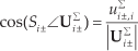
where i represents the x-, y- or z-axis and u _{i ±}, _i ^Σ represents the x, y or z elements of the vector U ^Σ _{i ±}. The resulting projection S_i±⊥ of the surface S_i± in the direction U Σ _{i ±} is given as

$S_{i\pm \perp }=S_{i\pm }\cos (S_{i\pm }\angle U_{i\pm }^{\sum })=S_{i\pm }\frac{u_{i\pm ,i}^{\sum }}{\left|U_{i\pm }^{\sum }\right|}$

(12)

Because S_i+= S_i- = S_i, it is possible to substitute (12) into equation (10) and to rewrite

$F_{i\pm }=\frac{1}{2}\rho C_{i\pm }{S}_i\frac{u_{i\pm ,i}^{\sum }}{\left|U_{i\pm }^{\sum }\right|}{\left|U_{i\pm }^{\sum }\right|}^2=\frac{1}{2}\rho C_{i\pm }{S}_i{u}_{i\pm ,i}^{\sum }\left|U_{i\pm }^{\sum }\right|$

(13)

where C_i± represents the correction parameter which includes the resistance coefficient (the drag coefficient). This correction parameter corresponds with surface S_i± and also considers the deviation of real flight behaviour from the model predictions (which is caused by accepting some of the simplifying assumptions mentioned above).

Here, it is necessary to explain how, in the PEM sense, F_i± represents the specific aerodynamic force from which the “drag” and “lift” effects can be derived. The “drag” and “lift” effects can be calculated by a specific aerodynamic force transformation (between two coordinate frame systems). Let F_i± be the aerodynamic force with respect to the projection surface S_i±⊥ which is orthogonal to the direction of the streamlines. Let the direction of the specific force F_i± (from which the “drag” and “lift” effects can be obtained by transformation) be orthogonal to the real surface direction S_i±, as shown in “Fig. 7”. Based on these relations, it is possible to create a regression model for aerodynamic forces with “drag” and “lift” effects. “Fig. 7” presents an example of a plate of the flight system which is exposed to airflow. In this example, the “drag” and “lift” effects are defined in frame system A and both are determined by the transformation of the specific force F_y- from frame system B (related to the plate surface) to frame system A (related to airflow). For any specific force balance of the surface S_i, it is possible to state that F_i = F_i+ + F_i-, which means

Figure 7.

The projection surfaces S_y-⊥ and S_y+⊥ and force F_y- for a plate (e.g., a flap)

$F_i=\frac{1}{2}\rho C_{i+}{S}_i{u}_{i+,i}^{\sum }\left|U_{i+}^{\sum }\right|+\frac{1}{2}\rho C_{i-}{S}_i{u}_{i-,i}^{\sum }\left|U_{i-}^{\sum }\right|=\frac{1}{2}\rho S_i\left(C_{i+}{u}_{i+,i}^{\sum }\left|U_{i+}^{\sum }\right|+C_{i-}{u}_{i-,i}^{\sum }\left|U_{i-}^{\sum }\right|\right)$

(14)

where

$\left|U_{i+}^{\sum }\right|=\sqrt{{\left(u_{i+\text{,x}}^{\sum }\right)}^2+{\left(u_{i+,y}^{\sum }\right)}^2+{\left(u_{i+\text{,z}}^{\sum }\right)}^2}\text{and}\left|U_{i-}^{\sum }\right|=\sqrt{{\left(u_{i-,\mathrm{x}}^{\sum }\right)}^2+{\left(u_{i-,\mathrm{y}}^{\sum }\right)}^2+{\left(u_{i-,\mathrm{z}}^{\sum }\right)}^2}$

The vector of the specific aerodynamic force F which acts on the body is given as (15)

$F=\frac{1}{2}\rho \left(\begin{array}{c}{S}_{\mathrm{x}}\left(C_{\mathrm{x}+}{u}_{\mathrm{x}+,\mathrm{x}}^{\sum }\sqrt{{\left(u_{\mathrm{x}+\text{,x}}^{\sum }\right)}^2+{\left(u_{\mathrm{x}+\text{,y}}^{\sum }\right)}^2+{\left(u_{\mathrm{x}+\text{,z}}^{\sum }\right)}^2}+C_{\mathrm{x}-}{u}_{\mathrm{x}-\text{,x}}^{\sum }\sqrt{{\left(u_{\mathrm{x}-\text{,x}}^{\sum }\right)}^2+{\left(u_{\mathrm{x}-\text{,y}}^{\sum }\right)}^2+{\left(u_{\mathrm{x}-\text{,z}}^{\sum }\right)}^2}\right)\\ S_{\mathrm{y}}\left(C_{\mathrm{y}+}{u}_{\mathrm{y}+,\mathrm{y}}^{\sum }\sqrt{{\left(u_{\mathrm{y}+\text{,x}}^{\sum }\right)}^2+{\left(u_{\mathrm{y}+\text{,y}}^{\sum }\right)}^2+{\left(u_{\mathrm{y}+\text{,z}}^{\sum }\right)}^2}+C_{\mathrm{y}-}{u}_{\mathrm{y}-\text{,y}}^{\sum }\sqrt{{\left(u_{\mathrm{y}-\text{,x}}^{\sum }\right)}^2+{\left(u_{\mathrm{y}-\text{,y}}^{\sum }\right)}^2+{\left(u_{\mathrm{y}-\text{,z}}^{\sum }\right)}^2}\right)\\ S_{\mathrm{z}}\left(C_{\mathrm{z}+}{u}_{\mathrm{z}+,\mathrm{z}}^{\sum }\sqrt{{\left(u_{\mathrm{z}+\text{,x}}^{\sum }\right)}^2+{\left(u_{\mathrm{z}+\text{,y}}^{\sum }\right)}^2+{\left(u_{\mathrm{z}+\text{,z}}^{\sum }\right)}^2}+C_{\mathrm{z}-}{u}_{\mathrm{z}-\text{,z}}^{\sum }\sqrt{{\left(u_{\mathrm{z}-\text{,x}}^{\sum }\right)}^2+{\left(u_{\mathrm{z}-\text{,y}}^{\sum }\right)}^2+{\left(u_{\mathrm{z}-\text{,z}}^{\sum }\right)}^2}\right)\end{array}\right)$

(15)

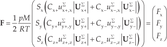
If equation (15) is substituted by the air density ρ = pM/RT where p is the atmospheric pressure, M is the air molecular weight, R is the universal gas constant and T is the air temperature, then it can be rewritten as

$F=\frac{1}{2}\frac{pM}{RT}\left(\begin{array}{c}{S}_{\mathrm{x}}\left(C_{\mathrm{x}+}{u}_{\mathrm{x}+,\mathrm{x}}^{\sum }\left|U_{\mathrm{x}+}^{\sum }\right|+C_{\mathrm{x}-}{u}_{\mathrm{x}-\text{,x}}^{\sum }\left|U_{\mathrm{x}-}^{\sum }\right|\right)\\ S_{\mathrm{y}}\left(C_{\mathrm{y}+}{u}_{\mathrm{y}+,\mathrm{y}}^{\sum }\left|U_{\mathrm{y}+}^{\sum }\right|+C_{\mathrm{y}-}{u}_{\mathrm{y}-\text{,y}}^{\sum }\left|U_{\mathrm{y}-}^{\sum }\right|\right)\\ S_{\mathrm{z}}\left(C_{\mathrm{z}+}{u}_{\mathrm{z}+,\mathrm{z}}^{\sum }\left|U_{\mathrm{z}+}^{\sum }\right|+C_{\mathrm{z}-}{u}_{\mathrm{z}-\text{,z}}^{\sum }\left|U_{\mathrm{z}-}^{\sum }\right|\right)\end{array}\right)=\left(\begin{array}{c}{F}_{\mathrm{x}}\\ F_{\mathrm{y}}\\ F_{\mathrm{z}}\end{array}\right)$

(16)

f. Correction parameters

As mentioned above, the PEM uses simplified equations which in general do not correspond exactly with the real airflow processes. The above-mentioned deviations of the dynamical model derived by the PEM can be successfully compensated for by use of the correction parameters C_i±. These correction parameters include the resistance coefficients and also respect the deviation of the specific sum velocity U _{i ±}^Σ from the real state of the system caused by all the simplifying assumptions that have been made [12]. Under the assumption that

$U_{i\pm }^{\sum }\left(\text{real}\right)=k_{1i\pm }{U}_{i\pm }^{\sum }\text{and}{F}_{i\pm }\left(\text{real}\right)=k_{2i\pm }{F}_{i\pm }$

where U ^Σ _{i ±}(real) is the real sum velocity and F_i±(real) is the real aerodynamic force, and if k_{1 i ±} and k_{2 i ±} are constant, then the correction parameter C_i± is given by

$C_{i\pm }=k_{2i\pm }{c}_{i\pm }{k}_{1\pm }^2$

where c_i± is a resistance coefficient corresponding to equation (10).

Consequently, it is possible to define the correctional parameters l_x, l_y and l_z, by which it becomes possible to consider any small discrepancies caused by any assumption about the orientation of a specific aerodynamic force F_i± (see “Fig. 7”). The original aerodynamic force F can be determined by equation (16), and so it is feasible to adjust this force by the following equations,

$G=\left(\begin{array}{c}{l}_{\mathrm{x}}\\ l_{\mathrm{y}}\\ l_{\mathrm{z}}\end{array}\right)\cdot F=\frac{1}{2}\frac{pM}{RT}\left(\begin{array}{c}{l}_{\mathrm{x}}\\ l_{\mathrm{y}}\\ l_{\mathrm{z}}\end{array}\right)\cdot \left(\begin{array}{c}{S}_{\mathrm{x}}\left(C_{\mathrm{x}+}{u}_{\mathrm{x}+,\mathrm{x}}^{\sum }\left|U_{\mathrm{x}+}^{\sum }\right|+C_{\mathrm{x}-}{u}_{\mathrm{x}-\text{,x}}^{\sum }\left|U_{\mathrm{x}-}^{\sum }\right|\right)\\ S_{\mathrm{y}}\left(C_{\mathrm{y}+}{u}_{\mathrm{y}+,\mathrm{y}}^{\sum }\left|U_{\mathrm{y}+}^{\sum }\right|+C_{\mathrm{y}-}{u}_{\mathrm{y}-\text{,y}}^{\sum }\left|U_{\mathrm{y}-}^{\sum }\right|\right)\\ S_{\mathrm{z}}\left(C_{\mathrm{z}+}{u}_{\mathrm{z}+,\mathrm{z}}^{\sum }\left|U_{\mathrm{z}+}^{\sum }\right|+C_{\mathrm{z}-}{u}_{\mathrm{z}-\text{,z}}^{\sum }\left|U_{\mathrm{z}-}^{\sum }\right|\right)\end{array}\right)$

where G is the corrected aerodynamic force, which is fine-tuned by the correction parameters l_x, l_y and l_z considering the case that | G | = | F |.

All the adjustment parameters mentioned above (such as C_i± and l_x, ly and l_z) can be determined for each airship part on the basis of experimental measurements during a real airship flight.

5. The balance of aerodynamic forces and the momentums for airship parts

a. Rudder balance

Let us consider the rudder parameters first. Here, it is possible to obtain a rudder balance with respect to the foregoing considerations. For the fixed body of the rudder, it is given that

$F_{\text{RP}}^{\text{AN}}=\frac{1}{2}\frac{pM}{RT}\left(\begin{array}{c}0\\ S_{\mathrm{y}}^{\text{RP}}{C}_{\mathrm{y}}^{\text{RP}}\left(u_{\mathrm{y}+,\mathrm{y}}^{\text{RP}\sum }\left|U_{\mathrm{y}+}^{\text{RP}\sum }\right|+u_{\mathrm{y}-,\mathrm{y}}^{\text{RP}\sum }\left|U_{\mathrm{y}-}^{\text{RP}\sum }\right|\right)\\ 0\end{array}\right)$

(17)

It can be considered that C_y+^RP =C_y-^RP =C_y^RP. On the basis of equations (3) and (4), the specific sum velocities U _y+^RPΣ and U _y-^RPΣ can be rewritten as U^RPΣ_y± =f(V ^RP, W) and the momentum of the specific aerodynamic force F _RP^AN is then given by $Q_{\text{RP}}^{\text{AN}}=R^{\text{RP}}\times F_{\text{RP}}^{\text{AN}}$ .

For the rudder flap (the rudder thickness is neglected), the balance conditions are similar as for the rudder fixed body. First, let us define the specific aerodynamic forces in the rudder flap body frame K as

$F_{\text{RA}}^{\text{AN}}\left(\mathrm{K}\right)=\frac{1}{2}\frac{pM}{RT}\left(\begin{array}{c}0\\ S_{\mathrm{y}}^{\text{RA}}\left(\mathrm{K}\right)C_{\mathrm{y}}^{\text{RA}}\left(u_{\mathrm{y}+,\mathrm{y}}^{\text{RA}\sum }\left(\mathrm{K}\right)\left|U_{\mathrm{y}+}^{\text{RA}\sum }\left(\mathrm{K}\right)\right|+u_{\mathrm{y}-,\mathrm{y}}^{\text{RA}\sum }\left(\mathrm{K}\right)\left|U_{\mathrm{y}-}^{\text{RA}\sum }\left(\mathrm{K}\right)\right|\right)\\ 0\end{array}\right)=\left(\begin{array}{c}0\\ F_{\text{RA}}^{\text{AN}}{\left(\mathrm{K}\right)}_{\mathrm{y}}\\ 0\end{array}\right)$

(18)

Here, it is considered that C_y+^RA=C_y-^RA=C_y^RA, and the specific sum velocities U _y+^RAΣ(K) and U_y-^RAΣ(K) are given on the basis of equations (3) and (4) where U _y+^RAΣ(K) = f(V ^RA(K), W (K)). Here, a specific force F^AN_RA(K) transformation from the rudder flap body frame K to the airship body frame is necessary, which is governed by the following equation,

$F_{\text{RA}}^{\text{AN}}=F_{\text{RA}}^{\text{AN}}{\left(\mathrm{K}\right)}_{\mathrm{y}}{\left(\begin{array}{ccc}-\sin \epsilon & \cos \epsilon & 0\end{array}\right)}^{\mathrm{T}}$

(19)

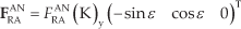
The momentum of the specific aerodynamic force F^AN_RA is then given as

$Q_{\text{RA}}^{\text{AN}}=R^{\text{RA}}\times F_{\text{RA}}^{\text{AN}}$

(20)

b. Elevators' balance — left and right elevators' fixed body (without a flap)

The elevators' balance is calculated separately for the left elevator's fixed body and flap and for the right elevator's fixed body and flap.

On the basis of the parameters for the left and right elevators' fixed body (the elevators' fixed body thickness is neglected), it is possible to provide the left and right elevators' fixed body balance with respect to the foregoing considerations. First, we define a specific aerodynamic force in left and right elevators' fixed body frames E⁺ and E⁻ as (21) and (22)

$F_{\text{EP}+}^{\text{AN}}\left({\mathrm{E}}^{+}\right)=\frac{1}{2}\frac{pM}{RT}\left(\begin{array}{c}0\\ 0\\ S_{\mathrm{z}}^{\text{EP}}\left({\mathrm{E}}^{\pm }\right)C_{\mathrm{z}}^{\text{EP}}\left(u_{\mathrm{z}+,\mathrm{z}}^{\text{EP}\sum }\left({\mathrm{E}}^{+}\right)\left|U_{\mathrm{z}+}^{\text{EP}\sum }\left({\mathrm{E}}^{+}\right)\right|+u_{\mathrm{z}-,\mathrm{z}}^{\text{EP}\sum }\left({\mathrm{E}}^{+}\right)\left|U_{\mathrm{z}-}^{\text{EP}\sum }\left({\mathrm{E}}^{+}\right)\right|\right)\end{array}\right)=\left(\begin{array}{c}0\\ 0\\ F_{\text{EP}+}^{\text{AN}}{\left({\mathrm{E}}^{+}\right)}_{\mathrm{z}}\end{array}\right)$

(21)

$F_{\text{EP}-}^{\text{AN}}\left({\mathrm{E}}^{-}\right)=\frac{1}{2}\frac{pM}{RT}\left(\begin{array}{c}0\\ 0\\ S_{\mathrm{z}}^{\text{EP}}\left({\mathrm{E}}^{\pm }\right)C_{\mathrm{z}}^{\text{EP}}\left(u_{\mathrm{z}+,\mathrm{z}}^{\text{EP}\sum }\left({\mathrm{E}}^{-}\right)\left|U_{\mathrm{z}+}^{\text{EP}\sum }\left({\mathrm{E}}^{-}\right)\right|+u_{\mathrm{z}-,\mathrm{z}}^{\text{EP}\sum }\left({\mathrm{E}}^{-}\right)\left|U_{\mathrm{z}-}^{\text{EP}\sum }\left({\mathrm{E}}^{-}\right)\right|\right)\end{array}\right)=\left(\begin{array}{c}0\\ 0\\ F_{\text{EP}-}^{\text{AN}}{\left({\mathrm{E}}^{-}\right)}_{\mathrm{z}}\end{array}\right)$

(22)

where it is considered that C_Z+^EP=C_z-^EP=C_z^EP. For specific sum velocities U _Z+^EPΣ(E⁺), U_Z-^EPΣ(E⁺) and U _Z+^EPΣ(E⁻), U _Z-+^EPΣ(E⁻) derived on the basis of equations (8), it can be summarized that U _Z±^EPΣ(E⁺) = f(V ^EP+(E⁺),W (E+)) and U_Z±^EPΣ)(E⁺) = f(V ^EP-(E⁻), W (E⁻)).

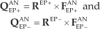
Next, the specific forces F _EP+^AN(E⁺) and F_EP-AN(E⁻) have to be transformed from the left and right elevators' fixed body frame E⁺ and E⁻ to the airship body frame by the following equations,

$\begin{array}{l}{F}_{\text{EP}+}^{\text{AN}}=F_{\text{EP}+}^{\text{AN}}{\left({\mathrm{E}}^{+}\right)}_{\mathrm{z}}{\left(\begin{array}{ccc}0& -\sin {\eta }^{+}& \cos {\eta }^{+}\end{array}\right)}^{\mathrm{T}}\text{and}\\ F_{\text{EP}-}^{\text{AN}}=F_{\text{EP}-}^{\text{AN}}{\left({\mathrm{E}}^{-}\right)}_{\mathrm{z}}{\left(\begin{array}{ccc}0& -\sin {\eta }^{-}& \cos {\eta }^{-}\end{array}\right)}^{\mathrm{T}}\end{array}$

(23)

The momentums of the specific aerodynamic forces F ^AN_EP+ and F ^AN_EP- are then given by

$\begin{array}{l}{Q}_{\text{EP}+}^{\text{AN}}=R^{\text{EP}+}\times F_{\text{EP}+}^{\text{AN}}and\\ Q_{\text{EP}-}^{\text{AN}}=R^{\text{EP}-}\times F_{\text{EP}-}^{\text{AN}}\end{array}$

(24)

c. Elevators' balance — left and right elevators' flap (without a fixed body)

On the basis of the parameters for the left and right elevators' flap (the elevator flap thickness is neglected), it is possible to provide the left and right elevators' flap balance with respect to the foregoing considerations. First, a specific aerodynamic force is defined in the left and right elevator flaps' body frames E⁺_μ and E⁻_σ as (25) and (26)

$F_{\text{EA}+}^{\text{AN}}\left({\mathrm{E}}_{\text{μ}}^{+}\right)=\frac{1}{2}\frac{pM}{RT}\left(\begin{array}{c}0\\ 0\\ S_{\mathrm{z}}^{\text{EA}}\left({\mathrm{E}}_{\text{μ|}\sigma }^{\pm }\right)C_{\mathrm{z}}^{\text{EA}}\left(u_{\mathrm{z}+,\mathrm{z}}^{\text{EA}\sum }\left({\mathrm{E}}_{\text{μ}}^{+}\right)\left|U_{\mathrm{z}+}^{\text{EA}\sum }\left({\mathrm{E}}_{\text{μ}}^{+}\right)\right|+u_{\mathrm{z}-,\mathrm{z}}^{\text{EA}\sum }\left({\mathrm{E}}_{\text{μ}}^{+}\right)\left|U_{\mathrm{z}-}^{\text{EA}\sum }\left({\mathrm{E}}_{\text{μ}}^{+}\right)\right|\right)\end{array}\right)=\left(\begin{array}{c}0\\ 0\\ F_{\text{EA}+}^{\text{AN}}{\left({\mathrm{E}}_{\text{μ}}^{+}\right)}_{\mathrm{z}}\end{array}\right)$

(25)

$F_{\text{EA}-}^{\text{AN}}\left({\mathrm{E}}_{\text{σ}}^{-}\right)=\frac{1}{2}\frac{pM}{RT}\left(\begin{array}{c}0\\ 0\\ S_{\mathrm{z}}^{\text{EA}}\left({\mathrm{E}}_{\text{μ|}\sigma }^{\pm }\right)C_{\mathrm{z}}^{\text{EA}}\left(u_{\mathrm{z}+,\mathrm{z}}^{\text{EA}\sum }\left({\mathrm{E}}_{\text{σ}}^{-}\right)\left|U_{\mathrm{z}+}^{\text{EA}\sum }\left({\mathrm{E}}_{\text{σ}}^{-}\right)\right|+u_{\mathrm{z}-,\mathrm{z}}^{\text{EA}\sum }\left({\mathrm{E}}_{\text{σ}}^{-}\right)\left|U_{\mathrm{z}-}^{\text{EA}\sum }\left({\mathrm{E}}_{\text{σ}}^{-}\right)\right|\right)\end{array}\right)=\left(\begin{array}{c}0\\ 0\\ F_{\text{EA}-}^{\text{AN}}{\left({\mathrm{E}}_{\text{σ}}^{-}\right)}_{\mathrm{z}}\end{array}\right)$

(26)

For the specific sum velocities U _Z+^EAΣ(E⁺_μ), U _Z-^EAΣ(E⁺_μ) and U _Z+^EAΣ(E⁻_Σ), U _Z-^EAΣ(E⁻_Σ) deduced on the basis of equation (8), it is given that U_Z+ ^EAΣ(E⁺_μ) = f(V EA+(E⁺_μ), W (E⁺_μ)) and U_Z+ ^EAΣ(E⁻_σ) = f(V^EA-(E⁻_σ), W(E⁻_σ)).

This specific forces F ^AN_EA+(E_μ⁺) and F ^AN_EA-(E⁻_σ) are now transformed from the left and right elevators' flap body frames E⁺_μ and E⁻_σ to the airship's body frame by the following equation

$F_{\text{EA}+}^{\text{AN}}=F_{\text{EA}+}^{\text{AN}}{\left({\mathrm{E}}_{\mu }^{+}\right)}_{\mathrm{z}}\left(\begin{array}{c}\cos {\eta }^{+}\sin \mu \\ -\sin {\eta }^{+}\\ \cos {\eta }^{+}\cos \mu \end{array}\right)\text{and}{F}_{\text{EA}-}^{\text{AN}}=F_{\text{EA}-}^{\text{AN}}{\left({\mathrm{E}}_{\sigma }^{-}\right)}_{\mathrm{z}}\left(\begin{array}{c}\cos {\eta }^{-}\sin \sigma \\ -\sin {\eta }^{-}\\ \cos {\eta }^{-}\cos \sigma \end{array}\right)$

(27)

The momentums of the specific aerodynamic forces F ^AN_EA+ and F ^AN_EA- are then given as

$\begin{array}{l}{Q}_{\text{EA}+}^{\text{AN}}=R^{\text{EA}+}\times F_{\text{EA}+}^{\text{AN}}\text{and}\\ Q_{\text{EA}-}^{\text{AN}}=R^{\text{EA}-}\times F_{\text{EA}-}^{\text{AN}}\end{array}$

(28)

d. Airship hull balance

The total hull balance of the airship consists of partial balances for the S_x, S_y and S_z surfaces. On the basis of the measured parameters for S_x, Sy and S_z, the hull as balanced for these surfaces can be estimated with respect to the foregoing considerations. Let every surface part (corresponding with a particular quadrant) of the S_x, S_y or S_z projection surface be assigned with the symbol i. In the case of the S_x, Sy and S_z surfaces, it is consistent that Sⁱ_x, Sⁱ_y and Sⁱ_z are the partial surfaces which are defined in the i -th quadrant, Cⁱ_x+, Cⁱ_x-, Cⁱ_y+, Cⁱ_y- and Cⁱ_z+, Cⁱ_z- are the correctional parameters of the partial surfaces, U _x+ ^{i Σ}, U _x- ^{i Σ}, U _y+ ^{i Σ}, 'U _y- ^{i Σ} and U _z+ ^{i Σ}, U _z- ^{i Σ} are the specific sum velocities of the partial surfaces, R ⁱ _sx, R ⁱ _sy and R ⁱ _sz are the position vectors towards the geometrical centres of the partial surfaces, and V ⁱ _sx, V ⁱ _sy and V ⁱ _sz, are the translational velocities of the geometrical centres. Specific aerodynamic forces for the airship's hull are then given as

$F_{\mathrm{H}}^{\text{AN}}=\frac{1}{2}\frac{pM}{RT}\left(\begin{array}{c}{\displaystyle \sum _{i=\mathrm{I}}^{\text{IV}}{S}_{\mathrm{x}}^i\left(C_{\mathrm{x}+}^i{u}_{\mathrm{x}+\text{,x}}^{i\sum }\left|U_{\mathrm{x}+}^{i\sum }\right|+C_{\mathrm{x}-}^i{u}_{\mathrm{x}-\text{,x}}^{i\sum }\left|U_{\mathrm{x}-}^{i\sum }\right|\right)}\\ {\displaystyle \sum _{i=\mathrm{I}}^{\text{IV}}{S}_{\mathrm{y}}^i\left(C_{\mathrm{y}+}^i{u}_{\mathrm{y}+\text{,y}}^{i\sum }\left|U_{\mathrm{y}+}^{i\sum }\right|+C_{\mathrm{y}-}^i{u}_{\mathrm{y}-\text{,y}}^{i\sum }\left|U_{\mathrm{y}-}^{i\sum }\right|\right)}\\ {\displaystyle \sum _{i=\mathrm{I}}^{\text{IV}}{S}_{\mathrm{z}}^i\left(C_{\mathrm{z}+}^i{u}_{\mathrm{z}+\text{,z}}^{i\sum }\left|U_{\mathrm{z}+}^{i\sum }\right|+C_{\mathrm{z}-}^i{u}_{\mathrm{z}-\text{,z}}^{i\sum }\left|U_{\mathrm{z}-}^{i\sum }\right|\right)}\end{array}\right)=\left(\begin{array}{c}{\displaystyle \sum _{i=\mathrm{I}}^{\text{IV}}{F}_{\mathrm{x}}^i}\\ {\displaystyle \sum _{i=\mathrm{I}}^{\text{IV}}{F}_{\mathrm{y}}^i}\\ {\displaystyle \sum _{i=\mathrm{I}}^{\text{IV}}{F}_{\mathrm{z}}^i}\end{array}\right)$

(29)

where the specific sum velocities U _x+ ^{i Σ}, U _x- ^{i Σ}, U _y+ ^{i Σ}, U _y- ^{i Σ}, U _z+ ^{i Σ}, and U _z- ^{i Σ} are derived on the basis of equations (3 to 8)

$\begin{array}{l}{U}_{\mathrm{x}\pm }^{i\sum }=f\left(V_{\text{Sx}}^i,W\right)\text{and}{U}_{\mathrm{y}\pm }^{i\sum }=f\left(V_{\text{Sy}}^i,W\right)\text{and}\\ U_{\mathrm{z}\pm }^{i\sum }=f\left(V_{\text{Sz}}^i,W\right)\forall i=\text{I, II, III, IV}\end{array}$

(30)

The momentums of the specific aerodynamic force F ^AN_H are calculated as

$Q_{\mathrm{H}}^{\text{AN}}={\left(\begin{array}{ccc}{\displaystyle \sum _{i=\mathrm{I}}^{\text{IV}}\left(R_{\text{sx}}^i\times F_{\mathrm{x}}^i\right)}& {\displaystyle \sum _{i=\mathrm{I}}^{\text{IV}}\left(R_{\text{sy}}^i\times F_{\mathrm{y}}^i\right)}& {\displaystyle \sum _{i=\mathrm{I}}^{\text{IV}}\left(R_{\text{sz}}^i\times F_{\mathrm{z}}^i\right)}\end{array}\right)}^{\mathrm{T}}$

(31)

6. Complete mathematical model of the airship flight mechanics

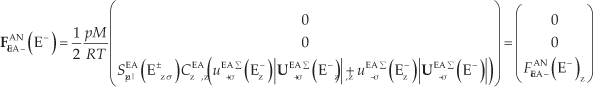
If the total aerodynamic force of the airship is designated as F ^AN and the total aerodynamic momentum of the airship as Q ^AN, then we can summarize as follows,

$F^{\text{AN}}=F_{\mathrm{H}}^{\text{AN}}+F_{\text{RP}}^{\text{AN}}+F_{\text{RA}}^{\text{AN}}+F_{\text{EP}+}^{\text{AN}}+F_{\text{EP}-}^{\text{AN}}+F_{\text{EA}+}^{\text{AN}}+F_{\text{EA}-}^{\text{AN}}$

(32)

$Q^{\text{AN}}=Q_{\mathrm{H}}^{\text{AN}}+Q_{\text{RP}}^{\text{AN}}+Q_{\text{RA}}^{\text{AN}}+Q_{\text{EP}+}^{\text{AN}}+Q_{\text{EP}-}^{\text{AN}}+Q_{\text{EA}+}^{\text{AN}}+Q_{\text{EA}-}^{\text{AN}}$

(33)

The mathematical model of the airship flight mechanics is obtained through Newton's mechanics, which are specifically adapted for this flight system (airship) and then combined with the balances of all the specific forces [2, 3, 13–19]. The aerodynamics part of this model corresponding with terms (32) and (33). The complete mathematical model of the airship flight mechanics is then given by

$\left(\begin{array}{cc}{M}_{11}& M_{12}\\ M_{21}& M_{22}\end{array}\right)\left(\begin{array}{c}\dot{V}\\ \dot{\mathrm{\Omega }}\end{array}\right)=\left(\begin{array}{c}{F}^{\mathrm{D}}\\ Q^{\mathrm{D}}\end{array}\right)+\left(\begin{array}{c}{F}^{\mathrm{G}}+F^{\mathrm{B}}+F_{\text{DHP}}^{\mathrm{T}}+F_{\mathrm{R}}^{\mathrm{T}}+F^{\text{AN}}\\ Q^{\mathrm{G}}+Q^{\mathrm{B}}+Q_{\text{DHP}}^{\mathrm{T}}+Q_{\mathrm{R}}^{\mathrm{T}}+Q^{\text{AN}}\end{array}\right)$

(34)

The meaning of these variables corresponds to [19] and [20]. The matrices M ₁₁, M ₁₂, M ₂₁ and M ₂₂ are components of the mass matrix, V = (v_x v_y v_z) ^T is the translational velocity vector, Ω = (ω_x ω_y ω_z) ^T is the angular velocity vector, F ^D and Q ^D are dynamic vector components, F ^G is the gravitation force vector, and F ^B is the buoyancy force vector. F ^T_DHP represents the dynamic thrust force vector of the main airship drive unit, F ^T_R is the thrust force vector of the rudder auxiliary propeller, and F ^AN is the aerodynamic force vector which is determined on the basis of the PEM (Terms 32 and 33) where Q ^G, Q ^B = (0 0 0)^T, Q ^T_DHP, Q ^T_R and Q ^AN are the momentums corresponding with these forces.

7. Model parameters

The parameters of the airship model (34) were determined on different tracks: the weight of the airship's constructional parts, the geometrical model obtained by airship photos and by 3D-CAD tools (here, “SolidWorks”), other experimental research such as Munk's correction factors [3], and identification from experimental airship flights. All the following values of the model parameters are valid only for a “nominal airship installation”. By a “nominal airship installation” is meant that the airship is considered to be well balanced (from the centre of rotation CR), including all necessary electronic components and auxiliary equipment (e.g., a video camera, specific sensors, etc.), and that it is ready for flight.

a. Constant airship parameters

1. Propulsion: The maximal static thrust of the main airship propulsion unit from which it is possible to determine the dynamical thrust F ^T_DHP, the position vector R _T of the main propulsion unit for which balanced thrust occurs, the maximal thrust F ^T_R of the rudder auxiliary propeller, and the position vector R _R of the rudder auxiliary propeller for balanced thrust.

2. Rudder: The projection surface S_y^RP of the fixed rudder body, the position vector R ^RP for the geometrical centre of the fixed rudder body projection surface, the projection surface S_y^RA(K) of the rudder flap, the position vector R ^RA for the geometrical centre of the rudder flap projection surface, the maximum range for the rudder flap angle ɛ_max.

3. Elevators: The projection surface S_z^EP(E^±) of the left and right elevators' fixed body, the position vectors R ^EP+ and R ^EP- for the geometrical centre of the left and right elevators' fixed body projection surfaces, the fixed constructional angle for the left and right elevators η⁺ and η⁻, the projection surfaces S_Z^EA(E^±_μ|σ) of the left and right elevators' flap, the position vectors R ^EA+ and R ^EA- for the geometrical centres of the left and right elevators' flap projection surfaces, the maximum range for the left and right elevators' flap angles μ_max and σ_max.

4. Airship hull: The partial projection surfaces Sⁱ_x, Sⁱ_y and Sⁱ_z, the position vectors for the airship hull's geometrical centres $R_{\text{sx}}^i$ , $R_{\text{sy}}^i$ , and $R_{\text{sz}}^i$ $\forall i=\text{I, II, III, IV}$ , and Munk's correctional factors f₁, f₂, f' [3].

b. Airship parameters valid for the “nominal airship installation”

Here belongs the centre of gravity R _CG, the airship weight without helium m_L, the helium weight m_He and the momentum of inertia matrix J.

c. Aerodynamic correctional parameters

The aerodynamic correctional parameters were determined by means of experimental airship flights. The first experimental flights had already been realized with closed-loop control. Different controllers were designed on the basis of the nominal mathematical model. Supported by additional experimental flights, the aerodynamic correctional parameters and the more advanced parameters for closed-loop control were determined. From this, more precise aerodynamic parameters were derived, which are considered in our fine-tuned mathematical model (34). All these aerodynamic parameters were determined under usual flight conditions, given as: wind of up to 1.5 m.s⁻¹, gusts of wind of up to 3.5 m.s⁻¹, the static thrust of the airship's main propulsion unit between 27.5 and 33.5 N, and the airship's cruise velocity between 4 and 10 m.s⁻¹.

The identification of the aerodynamic correction parameters was realized by the identification method “RMOCI” [21, 22], which was developed in our research group. This identification method can be characterized as a specific modification of the LDDIF (a form of least square method) method [23, 24] with respect to nonlinear state space models and based on nonlinear state space transformation [25]. Of course, the aerodynamic parameters can also be identified by several other identification methods, such as [20]. As such, the aerodynamic correction parameters are: for the fixed rudder body C_y+^RP = C_y-^RP = C_y^RP, for the rudder flap C_y+^RA =C_y-^RA =C_y^RA, for the left and right elevators' fixed body C_z+^EP =C_z-^EP =C_z^EP, for the left and right elevators' flap C_z+^EA =C_z^EA =C_z^EA, and for the airship hull $C_{\mathrm{x}+}^i=C_{\mathrm{x}-}^i$ , $C_{\mathrm{y}+}^i=C_{\mathrm{y}-}^i$ and $C_{\mathrm{z}+}^i=C_{\mathrm{z}-}^i$ $\forall i=\text{I,II,III,IV}$ .

On the basis of the results derived from simulations and experimental airship flights (see Chapter IX — Experimental comparisons), it becomes clear that is not necessary make use of the additional adaption parameters l_x, l_y and l_z (see Chapter IV/F – Correction parameters), which makes the identification process easier. Therefore, in our case, these parameters can be set as equal to 1.

8. Experimental comparisons

The experimental comparisons were carried out under usual flight conditions for an air temperature of 14 °C, for an air pressure of 102,250 Pa, and for the nominal airship setup with the static thrust of the airship drive unit as 33.5 N. In order to compare the experimental flights with our simulation results, we divided the experiments into two parts:

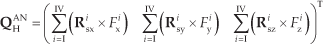
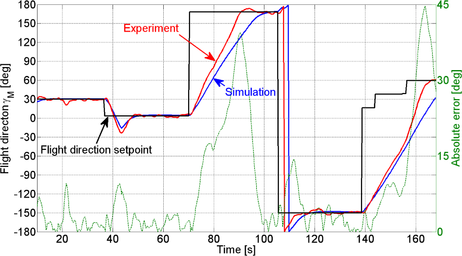
1. In the first part of the experimental flight, the airship control was adjusted to a constant flight altitude with changes in the flight direction only. The variable controller output for the airship flight direction is the rudder flap angle ɛ. During this part of our experimental flights, we analysed the following details: the form of the flight trajectory – “Fig. 8”, the airship flight direction – “Fig. 9” and the airship forwards velocity, see “Fig. 10”.

2. In the second part of the experimental flight, the airship flight controller already commands changes in the flight direction and the flight altitude at the same time. The controller outputs for this type of airship's experimental flight are the rudder flap angle ɛ and the elevators' flap angles μ and σ (the latter are controlled so that μ = σ holds at all times). During this part of the experimental flights, we compared the airship flight altitude – “Fig. 11”, the Euler angles – “Fig. 12” and the “Fig. 13”, airship translational velocity in the navigation frame (coordination system NED) – “Fig. 14”.

Figure 8.

Airship trajectory for the first part of the experimental flight

Figure 9.

Airship flight direction γ_M for the first part of the experimental flight

Figure 10.

Airship forward velocity V_F for the first part of the experimental flight

Figure 11.

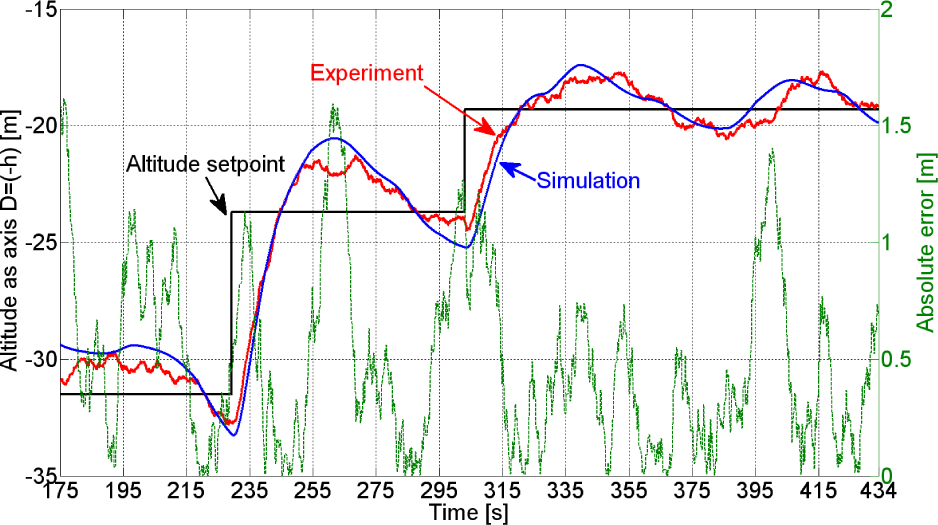
Airship flight altitude for the second part of the experimental flight

Figure 12.

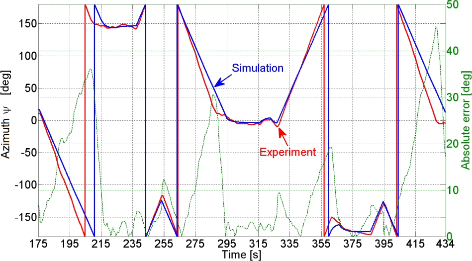
Euler angle yaw Ψ (azimuth) for the second part of the experimental flight

Figure 13.

Euler angle roll φ for the second part of the experimental flight

Figure 14.

Airship translational velocity v_N in the N-axis of the NED navigation frame for the second part of the experimental flight

The general problem for all the comparisons between the simulations and the experimental flights comprised unknown disturbances caused by gusts of wind. This problem lies in the fact that the direction of the gusts of wind which acted on the airship during the experimental flights could not be measured exactly, and so their impact could not be considered in comparing the simulations. For the simulation we accept the wind trends (as a replacement for gusts of wind).

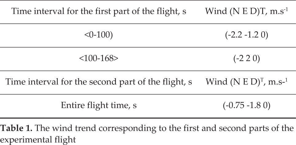
From this, in the simulation, the impact of gusts of wind was neglected and so it was not possible to compare all the state space values (such as for angular velocities), whereby the gusts of wind caused strong additional oscillations. It is due to this fact that it was possible to compare the Euler angles only. For all the simulations, the following wind trend was accepted (measured on the Earth's basis).

Table 1.

The wind trend corresponding to the first and second parts of the experimental flight

Time interval for the first part of the flight, s	Wind (N E D)T, m.s−1
<0–100)	(−2.2 −1.2 0)
<100–168>	(−2 2 0)
Time interval for the second part of the flight, s	Wind (N E D)T, m.s−1
Entire flight time, s	(−0.75 −1.8 0)

Simulations were carried out with the wind trend calculation only. Larger differences occur in the presented cases of the flight trajectory - “Fig. 8”, the airship forwards velocity - “Fig. 10” and the airship translational velocities – “Fig. 14”. The obvious reason for the larger difference in the case of the airship flight trajectory is the fact that any comparison of the 3D trajectories constitutes an extremely strong criterion. In the case considered here, small differences between the simulation and the experimental flight cause a continuous systematic growth of trajectory differences over time. The same applies for the airship forwards velocity, which is very sensitive to the wind trends and gusts of wind. Of course, the ideal conditions for comparison between the simulation and the experimental flight are given when the wind is calm. However, at our experimental site (located in the western part of Germany) it was necessary to accept windy flight conditions during our experimental comparisons. The results achieved are present in what follows.

The difference between the simulation and the experimental trajectories can be characterized by the average trajectory difference | ΔL̅ =43.8 m and by the corresponding average acceleration bias error ā = 0.34 mg, which is really a small difference (see “Fig. 8”). The difference between the flight directions can be characterized by an average flight direction difference | Δγ̄_M | = 8.3° (see “Fig. 9”). The difference between the airship forwards velocities can be characterized by an average airship forwards velocity difference | ΔV̄_F | = 0.7 m.s⁻¹ (see “Fig. 10”). Another difference between the simulation and the experimental flight courses can be described by the average flight altitude difference | Δh̄ | = 0.5 m (see “Fig. 11”). Another deviation between the simulation and the actual experimental course is given by the average yaw angle (azimuth) difference | Δψ̄ | = 10.6° (see “Fig. 12”). With respect to the “roll motion”, any deviation of values is considered by the average roll angle difference | Δφ | = 2° (see “Fig. 13”). For the “pitch motion”, the situation is the same as for the “roll motion” - any difference between the courses (simulation/experiment) can be nominated by the average pitch angle difference | Δθ | = 1.1°. Another difference between flight courses can be designated by the average translational velocity difference | Δv̄_N | = 1 m.s⁻¹ (see “Fig. 14”). For the translational velocity in the eastern direction, the situation is the same as for the translational velocity in the northern direction, and the difference between the flight courses can be characterized by the average translational velocity difference | Δv̄_E |= 0.9 m.s⁻¹.

9. Conclusion

In this article, the PEM is presented in general and applied specifically to an airship. With respect to the fact that airships are especially sensitive to airflow (e.g., wind), it is possible to prove the validity of this method by simulation and experimental flights under untoward conditions. On the basis of the results presented in this paper, it is shown that our PEM method can be applied for the computation of aerodynamic forces and momentums. The mathematical model obtained by the PEM proves the plausibility and reasonable dynamical behaviour of the flight system under consideration.

The main advantage of our PEM is that it provides a valid mathematical model framework with specific correction parameters which can be identified easily by measured data from experimental flights without complex or expensive experimental setups (e.g., wind tunnel measurement). The second advantage of the PEM is that its mathematical regression model, its internal structure and its descriptive extent are not too complicated for online applications on typical computer hardware, which can be carried by small flight systems. Its incorporated mathematical model is not demanding in terms of extensive CPU time, and so it is possible to apply this method in cases where it is necessary to calculate a continuous system state identification (e.g., to implement an adaptive control or a model predictive control, respectively).

On the basis of this mathematical model (presented in Eq. 34), we also designed an airship control system which allows us to compensate for airship oscillations about the x and y axes (roll and pitch, respectively) of the airship body frame. This compensation is a major advantage in many practical applications (such as on-board photography and video purposes). Some videos presenting the quality of the airship's dynamic flight behaviour in control mode are available here:

http://www.youtube.com/watch?v=sgIFKCPRpII

http://www.youtube.com/user/fernuniairship?features=results_main

Generally, the PEM may be applied to other UAVs as well (i.e., not only to airships) if it is possible to divide the UAV into specific constructional parts which can be considered to be relatively homogeneous from the aerodynamics viewpoint. Modelling methods comparable with the PEM are described in detail in [19] (an enhanced half-empirical airship model with force and momentum analyses of specific airship parts, such as the hull, the rudders and the elevators, and also a comparison with thin body theory) or in [26], which discusses the problem of small UAVs in wind.