Sage Journals: Discover world-class research

Abstract

Determining variations in fields is important for precision farming applications. Precision farming is used to determine, analyse, and manage factors such as temporal and spatial variability to obtain maximum profit, sustainability, and environmental protection. However, precision farming is excessively dependent on soil and plant test processes. Furthermore, test processes are time-consuming, laborious and expensive. These processes also cannot be performed quickly by humans. For these reasons, autonomous robots should be designed and developed for the detection of field variations and variable-rate applications. In this study, a remote-controlled and GPS-guided autonomous robot was designed and developed, which can be controlled via the 3G internet and is suitable for image-processing applications. The joystick is used to manually remotely control the robot movements in any direction or speed. Real-time video transmission to the remote computer can be accomplished with a camera placed on the vehicle. Navigation software was developed for steering the robot autonomously. In the results of the field test for the navigation software, it was found that the linear target point precision ranged from 10 to 12 cm and the distributed target point precision ranged from 15 to 17 cm.

Keywords

Remote Control GPS-guided Robot Navigation Precision Farming 3G Internet

1. Introduction

Agricultural practices have been revolutionized by the introduction of computers and electronic components. One example is automatic navigation of agricultural machines, including tractors and combine harvesters. GPS and machine vision techniques find many applications in agricultural production practices [1]. The developments of electronics and the resulting decrease in the size of computers, and the simultaneous development of smarter chips and microprocessors, have greatly affected the agricultural industry. Improvements in data acquisition and transfer and the processing power of computers, as well as their ability to process huge quantities of data in very little time, have contributed to the increase in autonomous vehicle research [2]. The potential benefits of automated agricultural vehicles include increased productivity and accuracy, together with enhanced operational safety. Research on autonomous agricultural vehicles has become very popular, and the robotics industry has developed a wide range of remarkable robots. In the near future, farmers will be using affordable, dependable autonomous vehicles for agricultural applications [3].

The historical development of the automatic tractor can be dated back to the early 20^th century. The first steering attachment for tractors was developed in 1924 [4]. Most agricultural machines that moved autonomously used mechanical settings until the 1970s. In the 1980s the potential for combining computers with image sensors provided opportunities for machine vision-based guidance systems [5]. Within 10 years, machine vision was being used to successfully guide agricultural tractors in the field [6, 7]. Around 1990, the Global Positioning System (GPS) became available in a limited capacity for civilian use, and the possibility of rapid and accurate vehicle location and navigation sparked a flurry of activity. In 1995, the system reached full operational capability; since that time, GPS has had a significant effect on agricultural practices [8]. In 1997, agricultural automation became a major issue, along with the advocacy of precision agriculture. Since 2000, drawing on developments in sensor and GPS technology, researchers have shown maintained interest in autonomous farm machinery.

Many research institutions have recently developed robot tractors and robot vehicles for agricultural purposes [9]. In [10] a sensor fusion technique for navigational posture estimation was developed for a skid-steered mobile robot vehicle in nursery tree plantations. In [11] an automated rice transplanter and autonomous guidance operation were developed. In [12] the authors developed a low-cost and small-scale electronic robot vehicle and automatic guidance system for orchard application. Another autonomous robot for use in orchards was developed in [13]: this vehicle is able to autonomously drive through tree rows. The researcher reported that the five vehicles completed so far have travelled autonomously over 300 km in research and commercial tree-fruit orchards; preliminary results in time trials conducted by extension educators indicate efficiency gains of up to 58%. Much further research has been performed towards the development of agricultural robot and semi-robot vehicles [14 –20].

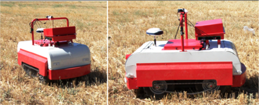
However, no study has yet reported on an autonomous vehicle that is both GPS-guided and remote-controlled, and which can be controlled via the internet for field applications. This study addresses this research gap (Figure 1). Navigation software is also developed for steering the robot autonomously.

Figure 1.

Remote-controlled and GPS-guided autonomous robot

2. Design of the autonomous robot

The designed robot is able to steer point to point both autonomously and under manual control. The robot involves five main sections:

Mechanical design and steering mechanism: An agricultural robot platform was developed to achieve the goal of both remote-controlled and autonomous navigation. The robot chassis, wheel module, and method of power are explained in this section.

Motor control mechanism: The mobile robot is a four-wheel robot which steers with two DC motors. The differential steering method is used. The DC motor controller and motor control algorithm are explained below.

Remote control algorithm: The joystick is used to manually remotely control the robot movements in any direction or speed. The data flow mechanism between the robot and the remote computer via the internet is explained in detail below.

Autonomous guidance algorithm: The GPS-guided robot is designed to operate in open field conditions. The GPS data processing and navigation algorithm are explained in this section, below.

Software development: Client-server software was developed to control all the functions in the robot. The running mechanism of the software is explained below.

2.1 Mechanical design and steering mechanism

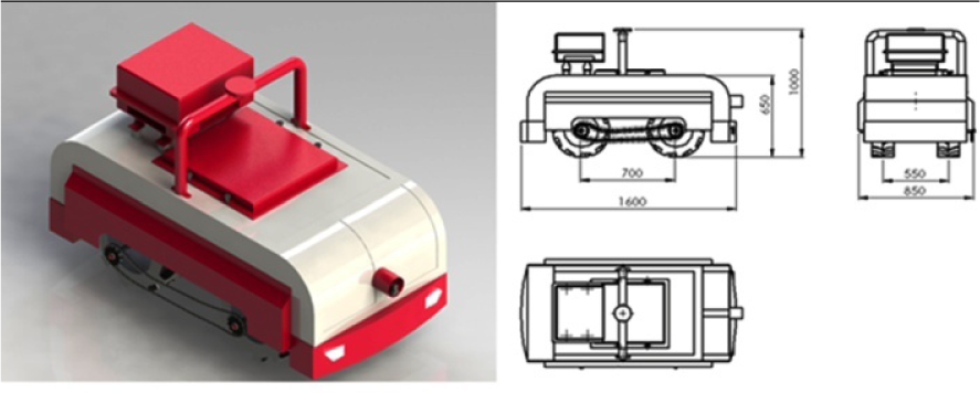
The designed robot is shown in Figure 2. The robot chassis was made of U-steel profile, and the body structure covered with sheet metal with a thickness of 2 mm. The robot was powered by two 24 V – 0.5 kW – 1440 rpm DC motors. Two reducers with 1:30 transmission rate were used to reduce rpm and increase torque. Four 4.00×8 agricultural rubber wheels were chosen to operate in open field conditions.

Figure 2.

Designed robot views

The DC motors and the front wheels were coupled to the reducers. The rear wheels were linked to each other with the help of the bearing shaft. A chain sprocket was mounted on each wheel, and the wheels on the right side and the left side were linked by the chain. This provided the differential steering mechanism (Figure 3). The steering system worked as follows: if the two motors rotate at the same speed, the robot moves forward or backward; if there is a difference between the speeds of the two motors, the robot steers in the direction of the slower motor.

Figure 3.

Designed robot views

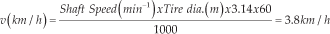
Energy input for the electronic components and the motors was provided by three 12 V, 72 Ah rechargeable maintenance-free sealed batteries. For the motors, two batteries were connected in series to provide 24 V. The other battery was connected to a DC/AC inverter. A12 V DC/AC inverter was used for the charge of the robot computer. The robot was able to continuously operate for six hours in the field. It weighed 250 kg and payload was approximately 900 kg. The reducer torque was calculated for each wheel according to Equation 1. The maximum robot speed was approximately 3.8 km/h (Equation 2).

R e d u c e r t o r q u e (N m) = \frac{M o t o r P o w e r (k W) * 9550}{R e d u c e r S p e e d (r e v / m i n)} = 99.5 N m

(1)

With an 8″ rim, the outside diameter of the wheel was approximately 440 mm. At a rated speed of 48 rev/min, the following vehicle speed was obtained:

v (k m / h) = \frac{S h a f t S p e e d (m i n^{- 1}) x T i r e d i a . (m) x 3.14 x 60}{1000} = 3.8 k m / h

(2)

The shaft torque can be calculated by Equation 3:

S h a f t t o r q u e = \frac{0.085 x W e i g h t (k g) x T i r e d i a . (m) x 9.8}{2} = 45.8 N m

(3)

The rolling resistance is very hard to determine. In the literature, rolling resistance coefficient = 0.085 is suggested for off-road (unpaved surface) applications.

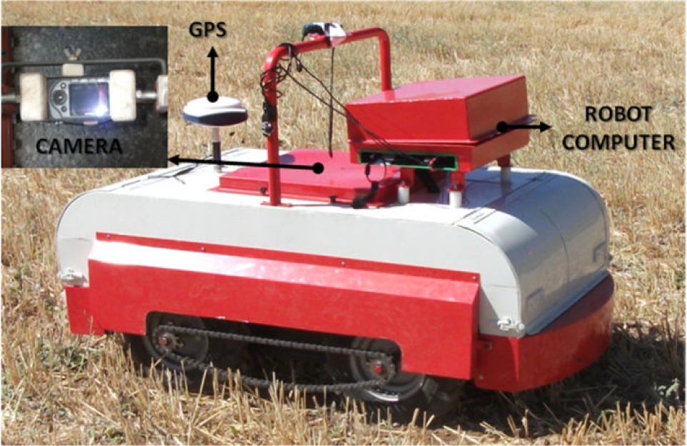
The developed robot was used to determine and map the stubble density ratio of a field using the online image-processing method. A Canon PowerShot SX100 IS digital camera mounted in a sealed box on the autonomous robot was used to obtain stubble images in the field. The base area of the sealed box was 45×50 cm. The digital camera was placed at a height of about 60 cm above the soil surface. The autonomous robot for stubble density measurement is shown in Figure 4.

Figure 4.

Developed robot for stubble density measurement

2.2 Mobile robot kinematics

The designed robot was assumed to be a nonholonomic system. Control of nonholonomic systems is theoretically challenging and practically interesting [21]. Although every nonholonomic system is controllable, it cannot be stabilized to a point with pure smooth (or even continuous) state feedback law because of Brockett's Theorem [22]. In order to overcome this difficulty, a variety of sophisticated feedback stabilization methods have been proposed by [21, 23–24].

To characterize the current localization of the mobile robot in its operational space of evolution on a 2D plane (x, y), we must first define its position and its orientation. Assume the angular orientation (direction) of a wheel is defined by angle θ between the instant linear velocity of the mobile robot v and the local vertical axis, as shown in Figure 5.

Figure 5.

The kinematics of the mobile robot

The translational velocities of the left and right wheels are obtained by v_L = ω_mlr/g and v_R = ω)_mrr/g, where ω_ml and ω_mr are angular speeds of the left and right drive motors, r the radius of the drive wheel, and g the reduction ratio of the reducer. The centre point P of the axle of the driving wheels is defined as the reference point of the mobile robot position. The forward linear velocity v and angular speed ω at the point P can be described in the moving frame as follows:

v = \frac{v_{R} + v_{L}}{2}

(4)

ω = \frac{v_{R} - v_{L}}{L}

(5)

where L is the distance between the two drive wheels. In the base frame, the kinematic model of the differential drive mobile robot can be expressed as:

(\begin{matrix} \dot{x} \\ \dot{y} \\ \dot{θ} \end{matrix}) = (\begin{matrix} c o s θ & 0 \\ s i n θ & 0 \\ 0 & 1 \end{matrix}) (\begin{matrix} v \\ ω \end{matrix})

(6)

where x, y, and θ are the positions and orientation of the robot and ẋ, ẏ, and θ̇ are their derivatives, representing the velocities and angular speed of the vehicle, respectively.

2.3 Motor control mechanism

A Roboteq AX3500 (Roboteq Inc., Arizona, USA) motor controller with two channel outputs was used to power and steer the robot by varying the speed and direction of the motors at each side of the chassis. The controller's two channels can be operated independently or combined to set the forward/reverse direction and steering of a robot by coordinating the motion on each side. The controller was designed to interface directly to high-power DC motors in computer-or remote-controlled mobile robotics and automated robot applications. The motors were driven using high-efficiency power MOSFET transistors controlled using Pulse Width Modulation (PWM) at 16 kHz. The AX3500 power stages can operate from 12 to 40 VDC and can sustain up to 60 A of controlled current, delivering up to 2400 W (approximately 3 HP) of useful power to each motor. The AX3500 motor controller was connected to the robot PC via its RS232 port. This connection can be used to both send commands and read various status information in real time from the controller. RS232 commands were very precise and securely acknowledged by the controller. The motor control mechanism block schema is given in Figure 6.

Figure 6.

Motor control mechanism block schema

Motor control software was developed for communication between the AX3500 controller and the robot computer. The robot computer's serial port was set as follows: 9600 bits/s, 7-bit data, 1 Start bit, 1 Stop bit, Even Parity. After connection, the controller was always ready to receive data and could send data from developed software at any time. The AX3500 used hexadecimal notation for accepting and responding to numerical commands. AX3500 motor control commands were composed of a series of four characters (Table 1). Motor speed value was sent from 00 to 7F in the forward or reverse direction for a given channel. These commands were sent to steer the robot both manually (joystick) and autonomously from the computer serial port using the developed software.

Table 1.

Motor speed commands and examples

	Control Sign	Command		Speed
	Control Sign	Motor 1	Motor 2	Motor 1	Motor 2
Motor Forward	!A00 – 7F	!A7F ↑	!A3F ↑	Forward-Fast	Forward-Slow
Motor Reverse	!a00 – 7F	!a3F ↓	!A7F ↑	Reverse-Slow	Forward-Fast
Motor Stop	!A00 or !a00	!A00	!a3F ↓	Stop	Reverse-Slow

2.4 Remote control algorithm

A Logitech Attack 3 joystick was used to control the robot. The joystick interfaced through a standard USB type-A connector to the remote computer. Software was developed to read the value of the two axes, and caused the robot to move accordingly. The y-axis controlled the forward-reverse movement of the robot, while the x-axis controlled the rotation left and right. Multiple button inputs could be configured for a variety of tasks. The program received x, y, and z values ranging from 0 to 65536 and also button values ranging from 1 to 11. Both axes were made proportional such that the speed of movement increased as the joystick moved a greater distance from the origin. Commands sent from the joystick were passed on by the remote computer at 10 ms intervals. Joystick commands are shown in Table 2.

Table 2.

Joystick commands

Control	Y-Axis		X-Axis
Control	Forward	Reverse	Right	Left
Joystick	32769 – 65536	0 – 32767	32769 – 65536	0 – 32767

There were some mismatches between motor-speed commands and joystick commands. For this reason, joystick commands were converted to motor-speed commands by the client software on the remote computer. The conversion table is given in Table 3. The buttons on the base of the joystick were assigned the following functions. Button 1 was emergency stop, which halted the system completely, requiring a restart both in autonomous and manual mode. Button 11 selected autonomous robot steering mode. Other buttons selected manual robot steering mode. The flow chart of the remote control algorithm of the robot is shown in Figure 7.

Table 3.

Conversation table between joystick and motor controller

Status	Motor Sign(MS)	Joystick sign(JS)	Proportioning
Motor Forward	!A00 – 7F	32769 – 65536	HEX(100 - FIX(JS / 330)) + 16
Motor Reverse	!a00 – 7F	0 – 32767	HEX(100 + (FIX(JS / 330) * −1)) − 16
Motor Stop	!A00 or !a00	32768	0

Figure 7.

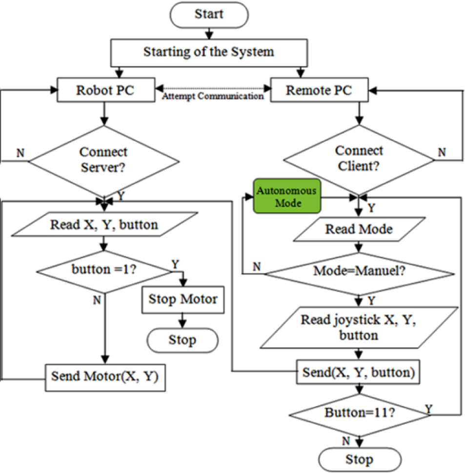
Robot remote control algorithm

2.5 Autonomous guidance algorithm

A Promark 500 GPS (Magellan Co., Santa Clara, CA, USA) receiver was used to navigate the robot. The receiver had 75 channels and up to 20 Hz data output rate. It was the most flexible GNSS (Global Navigation Satellite Systems) surveying system available, offering multiple operating modes, configurations and communication modules (UHF, GSM/GPRS, EDGE) and protocols. It was connected to Corse-TR (Continuously Operating Reference Stations-Turkey) via a phone data card (SIM Card) to receive correction signals. The receiver had a 99% confidence interval. The accuracy of the position obtained varied (according to the manufacturer's data) from below 10 mm with correction signals. The receiver had RS-232, Bluetooth, and USB ports to allow National Marine Electronics Association (NMEA) 0183 data transfer to a robot computer. Data such as the geographical coordinates and advance speed of the spot being measured were then sent to the serial port of the robot computer. The RS-232 serial communication protocol was used for two-way communication between the GPS receiver and the robot computer using the serial data cable of the GPS receiver. The GPS receiver installation data were sent to set up the GPS receiver via the server software [25].

In the robot, GPS receivers sent data on latitude, longitude, speed, time, etc., by cable to other electronic devices via the RS-232 serial port. NMEA 0183 was the standard protocol used by GPS receivers to transmit data. NMEA 0183 sentences were all American Standard Code for Information Interchange (ASCII). Each sentence was initiated with a dollar sign ($) and the next five characters determined the sentence type. The $GPRMC sentence type was the most useful format, and included positional and temporal data. The GPS receiver sent data every 10 ms to the software. The communication speed was set at 9600 baud. $GPRMC sentence fields were separated with commas. In the first step the sentence was stored in an array variable by the software; in the second step sentence fields were split by a Split command in the software, and in the third step positional data were converted to UTM (Universal Transverse Mercator) format and sentence fields stored to the SQL Server 2005 database (Figure 8).

Figure 8.

GPS data collection

A waypoint is the term used to describe a reference point for robot navigation. It includes destination latitude and longitude data. In this study, waypoints stored previously in the database were used for point-to-point steering in autonomous robot guidance. Two important angles called heading and azimuth angles were used to steer the robot autonomously. The heading angle was an angle between North (true or magnetic) and the current direction of the longitudinal axis of a robot in the horizontal plane. It was continuously received from the GPS receiver by the robot program. The azimuth was an angle between North and the destination point. It was continuously calculated by the robot program with Equation 7. The distance between the current robot location (X1, Y1) and the destination location (X2, Y2) was calculated with Equation 8.

A z i m u t h = A t a n 2 ((Y 2 - Y 1); (X 2 - X 1)) * 180 / π

(7)

D i s t a n c e = \sqrt{{(X 1 - X 2)}^{2} + {(Y 1 - Y 2)}^{2}}

(8)

In Equation 7, the Atan2 function returns the four-quadrant inverse tangent of (y/x) in the range -π ≤ return_val ≤ π, using the signs of both arguments to determine the quadrant of the return value. Y and X can be real-valued, signed or unsigned scalars, vectors, matrices, or N-dimensional arrays containing fixed-point angle values in radians.

The first stage of the autonomous guidance algorithm determined the angle difference by comparing the current heading to the target azimuth. This step allowed the robot to determine what direction (left or right) it should turn. The next step determined the distance between the robot location and the target location. The robot program continuously calculates the distance and the minimum turn required. When the heading angle is equal to the azimuth angle, the robot is steered towards the destination point. When the distance is equal to zero, the robot arrives at the destination point. The autonomous robot guidance algorithm is given in Figure 9.

Figure 9.

Autonomous robot guidance algorithm

Quadrant control was the most important factor for minimum robot turnings. The compass dial was divided into four quadrants. Angles were measured clockwise from North. Quadrant 1 was between 0 and 90 degrees, Quadrant 2 was between 90 and 180 degrees, Quadrant 3 was between 180 and 270 degrees, and Quadrant 4 was between 270 and 360 (or 0) degrees. The calculated azimuth angle (Equation 7) helped in determining the quadrant in which the target point was located. The heading angle of the robot helped in determining the quadrant in which the current point was located. The flowchart of the robot turning is given in Figure 10.

Figure 10.

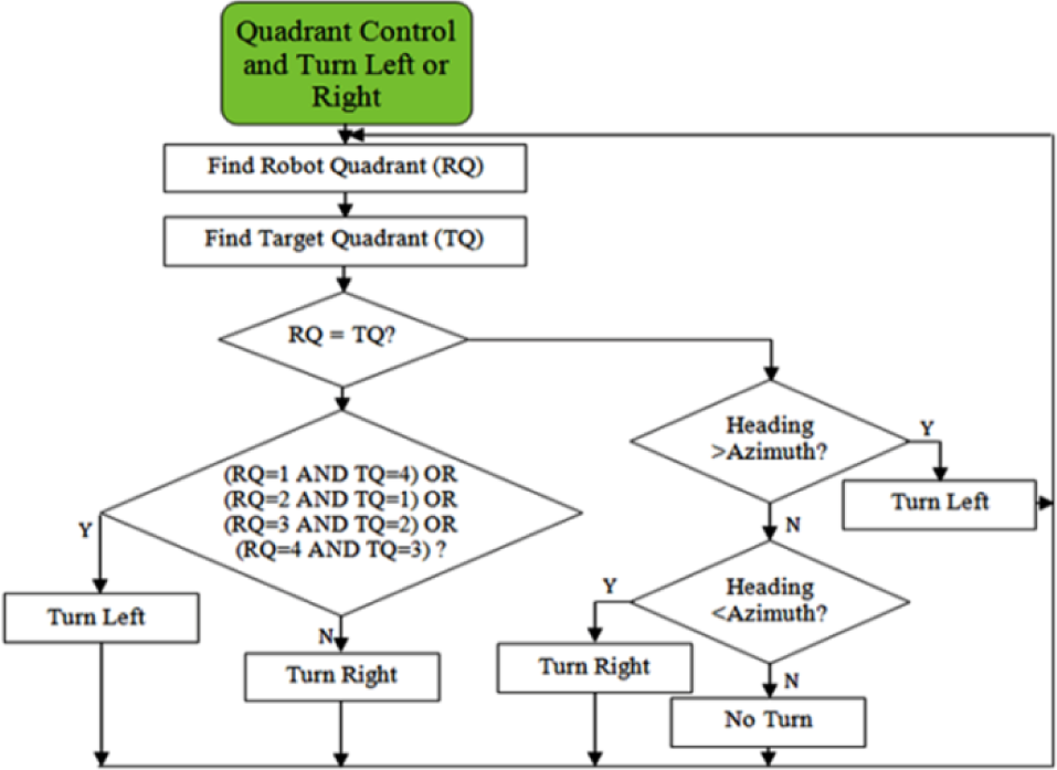
Flowchart of the robot turning

2.6 Software section

Two programs based on client/server architecture were developed to control and monitor the mobile robot. The server software was run on the robot computer (Figure 11).

Figure 11.

Developed server program

It was used to collect GPS data and perform steering. Collected data were stored to the database by the server program. The client program was run on the remote computer (Figure 12). It was used to manually control the robot and monitor the process data. Waypoints could be entered into the server software by the client program. In this way, a robot navigation file was created for autonomous operation. The developed client/server program was written in Microsoft Visual Basic.NET 2010. The communication between the robot and the remote computer was provided by a mobile 3G modem. The collected data were stored to a Microsoft SQL Server 2005 database.

Figure 12.

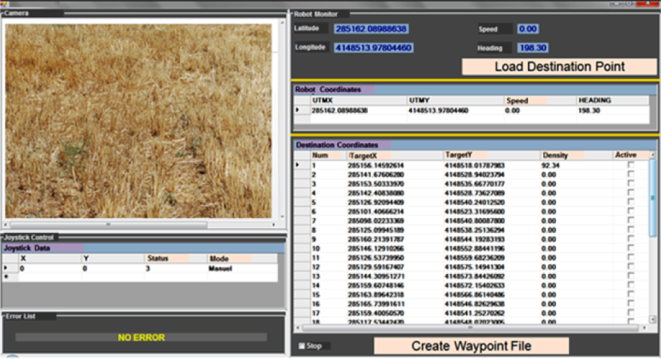
Developed client program

In this study, real-time video transmission to the remote computer was accomplished with a webcam camera placed on the vehicle. Yawcam™ surveillance software was installed on the vehicle computer as a video server. The video server could then send the video stream from the webcam through a specific port. In the developed system, as soon as the server software sends its IP address to the client software, video streaming starts between the vehicle computer and the remote computer. The 8080 port was used to provide video streaming for both computers.

In the server program, the image-processing algorithm was coded for determination of stubble density. All functions of the digital camera could be controlled by both the server software and the client software. The stubble images obtained by the server software were recorded to the robot computer. The obtained stubble density data were stored into the SQL Server database.

3. Experimental site

The field experiments were carried out in July 2012 in the agricultural experiment field of the West Mediterranean Agricultural Research Institute in Aksu, Antalya, located in the West Mediterranean region of Turkey. The research area was located approximately 20 km from Antalya between the coordinates 30°43′21″E and 36°52′39″N. The experimental field size was 2.4 ha, with wheat planted in June 2012. The ground situation was rough and slippery because of the wheat stubble.

4. Results and Discussion

A test procedure comprising two phases was performed to determine the accuracy of the robot in the field. In the first phase, linear offset errors were calculated. In linear calculation, the mobile robot was steered linearly from the start point (X1, Y1) to the destination point (X2, Y2). Each straight line was approximately 100 m long. This process was conducted 10 times at constant speed. Thereafter, offset distance error was measured between the robot stop point and the destination point with the help of a tape measure (Figure 13). The result of the linear calculation is given in Table 4.

Table 4.

Linear offset errors

Iteration	Distance(m)	Offset Error(cm)	Mean Error(cm)	Standard Deviation
1	100	10.30	11.32	0.92
2		11.20
3		10.70
4		10.50
5		12.00
6		11.00
7		13.00
8		12.50
9		10.50
10		11.50

Figure 13.

Determination of the linear offset error

In the second phase, the mobile robot was steered autonomously three times at 10 different points with different orientations relative to the destination point. Thereafter, the nonlinear offset distance error was measured between the robot stop point and the destination point with the help of a tape measure (Figure 14).

Figure 14.

Determination of nonlinear offset error

The linear offset error was found to be between 10.30 and 13 cm, and the nonlinear offset error between 13 and 20 cm. Standard deviation as calculated as 0.92 for the linear test and approximately 1.94 for the nonlinear test. The total maximum error of the robot navigation was estimated between 15 and 17 cm. The results of the nonlinear calculations are given in Table 5.

Table 5.

Linear offset errors

DestinationPoint No.	Iteration 1Offset Error(cm)	Iteration 2Offset Error(cm)	Iteration 3Offset Error(cm)
1	18.50	19.40	20.00
2	17.60	16.50	13.50
3	13.00	15.20	14.40
4	13.50	16.70	16.10
5	16.40	14.90	15.00
6	15.00	16.00	14.90
7	14.50	13.90	13.90
8	15.50	13.60	14.10
9	17.30	13.00	17.10
10	14.10	12.80	16.00

Mean Error (cm)	15.54	15.20	15.50
Standard Dev. (cm)	1.85	2.03	1.94

Various studies have been done on autonomous agricultural robots and guidance systems. In [2] the authors developed an inexpensive guidance system for use on a small agricultural vehicle suitable for soil testing purposes. The paper reported that the maximum error of offsets ranged from 3 to 6 m within the actual destination point for the developed system. The study reported in [11] developed an automated six-row rice transplanter and autonomous guidance system. The paper reported that the root mean square deviation from the desired straight path was approximately 5.5 cm and the maximum deviation from the desired path is less than 12 cm at 0.7 m/s operating speed. In [26] the authors developed an algorithm for improving the multi-path error in positioning systems by coupling a differential global positioning system (DGPS) and a double electric compass (DEC) in the navigation system of an orchard robotic vehicle. The researchers reported that the average distance error of the developed system was 17.5 cm for the straight line path and 22.3 cm for the U-turn path. The developed robot and navigation algorithm are therefore very useful for precision farming applications when compared to similar studies carried out by other researchers (Table 6).

Table 6.

Comparison table for similar studies

Literature	Performance Results
Stombaugh et al. [27]	Lateral position error at 4.5 m/s within 16 cm (95% confidence)
Nagasaka et al. [11]	Maximum deviation from the desired path less than 12 cm
Guo and Zhang [28]	With vehicle travelling in an open field area, maximum error was reduced to 0.30 m
Nistala [2]	Total maximum error of system estimated to be between 25 and 30 cm, including the Differential GPS error
Kanjanaphachoat et al. [26]	Positioning system had an average SD of 20.7 cm and an average distance error of 17.5 cm
Garcia et al. [29]	Error usually below 1 m

In this study, the robot navigation was provided fully by RTK-GPS data. GPS accuracy is the most important factor affecting the reliability of the robot position estimates and thus the navigation of the designed robot. If a GPS receiver with different accuracy is placed on the designed robot, navigation accuracy can change significantly. Mechanical changes could be made to the robot for better performance and manoeuvrability.

5. Conclusions

A remote-controlled and GPS-guided autonomous robot was successfully developed for use in precision farming applications in Turkey. The developed robot can steer point to point both autonomously and manually. Both linear and nonlinear offset error measurements were made. The developed robot's weight was 250 kg and the payload was approximately 900 kg. Because of the payload value, the robot can be used as a transport vehicle. The robot speed was approximately 3.8 km/h and the torque on each wheel was approximately 99.5 Nm. Considering these values, the developed robot can provide a high level of convenience for precision farming applications such as soil penetration measurement, soil sampling, and weed spraying. The robot can access remote computers via the internet (using a 3G modem). This makes it able to store/retrieve telemetry data to/from the remote computers. Further studies are needed to focus on adaptation of different sensors towards developing an intelligent robot.

Footnotes

6. Acknowledgements

This work was supported by The Scientific Research Projects Coordination Unit of Akdeniz University (project number: 2011.03.0121.011).

References

Andres

Design of an autonomous navigation system for a mobile robot [thesis]. Montreal: McGill University; 2005.

Nistala

. Development of an Inexpensive Guidance System for Agricultural Purposes [thesis]. Baton Rouge: Louisiana State University; 2006.

Imou

Wakabayashi

Yokoyama

Review of research on agricultural vehicle autonomous guidance. Int. J. Agric. & Biol. Eng. (IJABE). 2009; 2:1–16. DOI: 10.3965/j.issn.1934-6344.2009.03.001-016

Willrodt

. Steering attachment for tractors US Patent 1506706 [Internet]. 1924. Available from: http://www.freepatentsonline.com/1506706.pdf. Accessed on 12 Jan 2015.

Reid

Zhang

Noguchi

Dickson

Agricultural automatic guidance research in North America. Comput. Electron. Agr. 2000; 25(1–2):155–167. DOI: 10.1016/S0168-1699(99)00061-7

Gerrish

Fehr

Van

Welch

. Self-steering tractor guided by computer vision. Appl. Eng. Agric. 1997; 13(5)559–563. DOI: 10.13031/2013.21641

Reid

Searcy

. An Algorithm for Separating Guidance Information from Row Crop Images. Trans. ASAE. 1998; 31(6):1624–1632. DOI: 10.13031/2013.30910

Heraud

Lange

. Agricultural automatic vehicle guidance from horses to GPS: how we got here, and where we are going. In Proceedings of the Agricultural Equipment Technology Conference; 8–11 February 2009; USA. Louisville; 2009. p. 1–67.

Noguchi

Barawid

Robot farming system using multiple robot tractors in Japan Agriculture, Preprints of the 18th IFAC World Congress; 28 August-2 September 2011; Italy. Milan; 2011. p. 633–637.

10.

Khot

Tang

Blackmore

Nørremark

Navigational context recognition for an autonomous robot in a simulated tree plantation. Trans. ASABE. 2006; 49(5):1579–1588. DOI: 10.13031/2013.22032

11.

Nagasaka

Umeda

Kanetai

Taniwaki

Sasaki

Autonomous guidance for rice transplanting using global positioning and gyroscopes. Comput. Electron. Agr. 2004; 43(3):223–234. DOI: 10.1016J.COMP AG.2004.01.005

12.

Barawid

Jr Noguchi

Development of low-cost and small-scale electronic robot vehicle. Automatic Guidance System in Real-time Orchard Application (Part 2). J. Soc. Agric. Machinery. 2010; 72(3):243–250. DOI: 10.11357/JSAM.72.243

13.

Bergerman

Singh

Hamner

Results with autonomous vehicles operating in specialty crops. IEEE International Conference on Robotics and Automation; 14–18 May 2012; USA. Minnesota; 2012. p. 1829–1835.

14.

Gerrish

Surbrook

Mobile robots in agriculture. Robotics and Intelligent Machines in Agriculture: Proceedings of the First International Conference on Robotics and Intelligent Machines in Agriculture; 2–4 October 1983; USA. St. Joseph; 1983. p. 30–41.

15.

Debain

Chateau

Berducat

Martinet

Bonton

A guidance-assistance system for agricultural vehicles. Comput. Electron. Agr. 2000; 25:29–51. DOI: 10.1016/S0168-1699(99)00054-X

16.

Han

Zhang

Noh

Sin

A dynamic performance evaluation method of DGPS auto guidance systems under linear parallel-tracking applications. Trans. ASAE. 2004; 47(1):321–329. DOI: 10.13031/2013.15857

17.

Pilarski

Happold

Pangels

Ollis

Fitzpatrick

Stentz

The demeter system for automated harvesting. Auton. Robot. 2002; 13:9–20. DOI: 10.1023/A:1015622020131

18.

Morimoto

Suguri

Umeda

Vision-based navigation system for autonomous transportation vehicle. Precis. Agric. 2005; 6:239–254. DOI: 10.1007/S11119-005-1384-X

19.

García-Pérez

García-Alegre

Ribeiro

An agent of behaviour architecture for unmanned control of a farming vehicle. Comput. Electron. Agr. 2008; 60:39–48. DOI: 10.1016/J.COMPAG 2007.06.004

20.

Subramanian

Burks

Arroyo

Development of machine vision and laser radar based autonomous vehicle guidance systems for citrus grove navigation. Comput. Electron. Agr. 2006; 53(2): 130–143. DOI: 10.1016/J.COMPAG.2006.06.001

21.

Chen

Robust stabilization for a class of dynamic feedback uncertain nonholonomic mobile robots with input saturation. Int. J. Control Autom. 2014; 12(6):1216–1224. DOI: 10.1007/S12555-013-0492-Z

22.

Brockett

. Asymptotic stability and feedback stabilization. In: Brockett

Millman

Sussmann

, editors. Differential Geometric Control Theory. Boston: Birkhauser; 1983. p. 181–208.

23.

Chen

Ding

Chen

Wang

Zhu

Chen

Global Finite-time Stabilization for Nonholonomic Mobile Robots Based on Visual Servoing. Int. J. Adv. Robot Syst. 2014; 11(180):1–13. DOI: 10.5772/59307

24.

Chen

Zhang

Chen

Global Practical Stabilization for Non-holonomic Mobile Robots with Uncalibrated Visual Parameters by Using a Switching Controller. IMA J. Math. Contr. Inform. 2013; 30:543–557. DOI: 10.1093/IMAMCI/DNS044

25.

Topakci

Unal

Canakci

Celik

Karayel

Design of a Horizontal Penetrometer for Measuring On-the-Go Soil Resistance. Sensors. 2010; 10:9337–9348. DOI: 10.3390/S101009337

26.

Kanjanaphachoat

Hsieh

Cheng

Mins-Shi

Combining a differential positioning system and double electric compass to improve multi-path error correction for a high-precision agricultural robotic vehicle. Maejo Int. J. Sci. Technol. 2011; 5(2): 169–180. WOS: 000298040700001

27.

Stombaugh

Benson

Hummel

. Guidance Control of Agricultural Vehicles at High Field Speeds. Transactions of the ASAE. 1999; 42(2): 537–544. DOI: 10.13031/2013.13387

28.

Guo

Zhang

A low-cost navigation system for autonomous off-road vehicles. In: Proceedings of Automation Technology for Off-road Equipment Conference (ASABE); 7–8 October 2004; Japan. Kyoto; 2004. p. 107–119. DOI: 10.13031/2013.17824

29.

Garcia

Gil

Arribas

. Evaluation of the use of low-cost GPS receivers in the autonomous guidance of agricultural tractors. Spanish Journal of Agricultural Research. 2011; 9(2):377–388. DOI: 10.5424/SJAR/20110902-088-10

Design of a Remote-Controlled and GPS-Guided Autonomous Robot for Precision Farming

Abstract

Keywords

1. Introduction

2. Design of the autonomous robot

2.1 Mechanical design and steering mechanism

2.2 Mobile robot kinematics

2.3 Motor control mechanism

2.4 Remote control algorithm

2.5 Autonomous guidance algorithm

2.6 Software section

3. Experimental site

4. Results and Discussion

5. Conclusions

Footnotes

6. Acknowledgements

References