Sage Journals: Discover world-class research

Abstract

A sliding mode control method based on radial basis function (RBF) neural network is proposed for the deburring of industry robotic systems. First, a dynamic model for deburring the robot system is established. Then, a conventional SMC scheme is introduced for the joint position tracking of robot manipulators. The RBF neural network based sliding mode control (RBFNN-SMC) has the ability to learn uncertain control actions. In the RBFNN-SMC scheme, the adaptive tuning algorithms for network parameters are derived by a Koski function algorithm to ensure the network convergences and enacts stable control. The simulations and experimental results of the deburring robot system are provided to illustrate the effectiveness of the proposed RBFNN-SMC control method. The advantages of the proposed RBFNN-SMC method are also evaluated by comparing it to existing control schemes.

Keywords

Sliding Mode Control (SMC)Radial Basis Function Neural Network (RBFNN)Radial Basis Function Neural Network Sliding Mode Control (RBFNN-SMC)Deburring Robotic Control

1. Introduction

The robotic deburring system was developed to replace labour-intensive and low-productivity manual operations in industry production. Burrs not only affect the surface quality and practical application of products, but can also be harmful to worker safety and the environment. Deburring robots can reduce the scrap rate of parts due to its automatic operation, flexible and intelligent control and high machining efficiency.

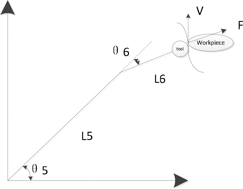
Burrs can be removed by controlling tangential force of tool, positional inaccuracies can be compensated for by controlling the normal force of tool. Burrs are removed from the edges of metal parts of different sizes and shapes and deburring efficiency is dependent on tool sharpness and cutting forces. A deburring process is required to remove burrs and to produce a chamfer for smoothing the edges of metal parts. When the force required to remove burrs is equal to or greater than the force required to chamfer, it becomes difficult to detect the deflection of the end-effector caused by disturbance, part misalignment and tool wear.

An efficient deburring algorithm is needed to solve the problems of both compensating for positional inaccuracies and adjusting the feed rate according to burr size. In reality, these parameters may vary due to changes in operational conditions; furthermore, these parameters are generally unknown, which results in impact during transition and a poor force tracking performance. A sliding mode control based on a neural network was therefore applied to deal with highly variable burrs.

Variable structure systems incorporating a sliding mode method were used to the robotic systems [1 –8] and conventional sliding mode controllers were designed to improve the robustness of robotic systems. Some experts have combined the control algorithm and conventional sliding mode method to solve the chattering phenomenon. The novel adaptive sliding mode controllers can adjust the control torque based on real-time position tracking errors, which alleviates the chattering phenomenon of the sliding mode controller [9 –14].

The combined control algorithm also reduced the output error and improved the performance of the robotic system. The fuzzy controller with sliding mode and online learning were designed to eliminate the steady-state error and improve the transient response performance of the systems [15 –17]. In order to ensure the stability of the system, Ruey-Jing Lian developed an adaptive self-organizing fuzzy sliding-mode radial basis-function neural-network controller for robotic systems [18]. The experimental results of this research showed that this method works better than the conventional sliding mode control method.

When a system is uncertain and exhibits disturbance, the mathematical model is difficult to create. Precision must be guaranteed and as a result, the robust sliding mode controllers were designed. Robust trajectory tracking, precise positioning and a robust hybrid intelligent control scheme were applied to the industrial robot [19 –22]. Problems were addressed in the presence of uncertainties and disturbances. The neural network based on a sliding mode control scheme and iterative learning controller was proposed for controlling robotic systems [23]. The experimental results showed that a neural network based on a sliding mode control scheme and ILC achieved better control performance compared to the conventional sliding mode control method [24].

A novel application of the bacterial foraging optimization algorithm (BFO) is presented in [25] and the simulation results show that the BFO algorithm is superior to the PSO algorithm in terms of response accuracy. Stable indirect adaptive control with recurrent neural networks (RNN) is presented for square multivariable non-linear plants with unknown dynamics [26] and experiment results show that this approach results in good performance, simple structure and self-tuning of parameters.

A fuzzy PID control strategy is presented in [27–28]. The fuzzy PID controller can apply an analysis in order to effect self-tuning via fuzzy logic, as well as proportional, derivative and integral gain matrices.

Additional algorithms have also been proposed [29 –31]. A subset selection algorithm considers the selected and remaining features; this approach can avoid the interference of relevant but redundant features and overcome the weakness of forward greedy search based methods [29]. A quick attribute reduction algorithm for a neighbourhood rough set model is proposed in [30]. An efficient and robust pose estimation algorithm for multi-camera systems that can obtain 6DOF poses for all cameras using only a few coplanar points simultaneously is proposed in [31]. Detection chain repeatability, average detection chain re-projection error and matching chain precision are presented in [32].

Nonetheless, despite the presence of a variety of algorithms, the uncertainty factor could not be diminished; therefore, the sliding mode control based on a RBF neural network is proposed. In this paper, a dynamic model is introduced and the control scheme has no strict system information requirements, no constraints, an accurate model and exact parameters. This paper is organized into five sections: following the introduction, section 2 presents the dynamic model of a two-link deburring robot manipulator. The actuator dynamics is analysed and the conventional SMC system for the dynamic model is proposed. In section 3, the sliding mode control is introduced and the sliding control system design is presented. In section 4, a RBF neural network based sliding-mode control (RBFNN-SMC) scheme is proposed, where a RBF neural network is combined with the SMC to relax the requirements of system parameters and sustain the robust features of robot manipulator. The RBFNN-SMC scheme is derived from a Koski function and its position accuracy control and trajectory tracking stability is guaranteed in the closed-loop control scheme. In section 5, simulations and experimental results of the deburring robot are presented in the presence of some uncertainties and interferences to demonstrate the robust control performance of the RBFNN-SMC scheme. Finally, conclusions are drawn in section 6.

2. Dynamic model of a 6-DOF deburring robot

The subject of this paper is a 6-DOF deburring robot, as shown in Fig.1. The dynamic model was created based on a simple structure.

Figure 1.

The simple structure of ER50-C20 robot

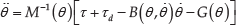
Considering a 6-DOF robot arm that takes into account friction forces and dynamic and nonlinear disturbances, the equation of motion is given by:

M (q) \ddot{q} + B (q, \dot{q}) + G (q) = τ + τ_{d}

(1)

where:

$M (q)$ is $n \times n$ inertia matrix, positive definite, decided by mass, velocity and length of the link i.

$B (q, \dot{q})$ is n×n inertia matrix and represents the centrifugal force generated by the motion of connected links.

$G (q)$ is n×1 inertia matrix and represents gravitational torques.

τ is input torques vector.

$τ_{d}$ is unknown disturbances including unstructured nonlinear dynamics.

The six joint variables of the robot are all rotational joints and therefore, $q = θ$ . In order to simplify the dynamic model, joints 5 and 6 should specifically be taken into account according to the working conditions. Links 5,6 of the robot manipulator and workpiece are modelled, as shown in Fig.2

Figure 2.

Cylinder head of motorcycle is polished by the terminal tool

Path planning to remove burrs on the cylinder head of the motorcycle needs to be established. the desired path is planned by workers and robot manipulator will follow this desired path, this process is an artificial teaching manner. Firstly, the workpiece is polished in an artificial teaching manner and the teaching path is obtained. This path will be recorded by the robot; additionally, the force and feed speed of this path will also be recorded to provide reference values for the next workpiece. After polishing the first workpiece, the desired joint angular displacement is obtained and is labelled θ_d. The next workpiece is polished to obtain actual joint angular displacement θ. The angular error is e=θ_d−θ.

The angular displacements of six joints can be given by θ=[θ₁,θ₂,θ₃,θ₄,θ₅,θ₆].

The torque is given as $τ = [τ_{1}, τ_{2}, τ_{3}, τ_{4}, τ_{5}, τ_{6}]$ .

The mechanical behaviour of a 6-DOF robot manipulator is considered and expressed by the following Lagrange equation:

L (θ, \dot{θ}) = E_{k} (θ, \dot{θ}) - E_{p} (θ)

(2)

The kinetic energy of link 6^th is given by:

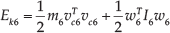
E_{k 6} = \frac{1}{2} m_{6} v_{c 6}^{T} v_{c 6} + \frac{1}{2} w_{6}^{T} I_{6} w_{6}

(3)

where

$E_{k} (θ, \dot{θ})$ = total kinetic energy generated by the movement of the robot.

$E_{p} (θ)$ = potential energy generated by the movement of the robot based on the base coordinate system.

$\frac{1}{2} m_{6} v_{c 6}^{T} v_{c 6}$ = kinetic energy generated by centroid linear speed of link 6.

$\frac{1}{2} w_{6}^{T} I_{6} w_{6}$ = kinetic energy generated by the angular speed of link 6.

The total kinetic energy is given by:

E_{k} = \sum_{i = 1}^{6} E_{k i}

(4)

The base coordinate system is regarded as the reference coordinate system and the potential energy of link 6 can be expressed as:

E_{p 6} = - m_{6} g^{T} p_{c 6}

(5)

g = 3×1 the vector of gravitational acceleration.

$p_{c 6}$ = centroid position vector of link 6.

The total potential can be given by:

E_{p} = \sum_{i = 1}^{6} E_{p i}

(6)

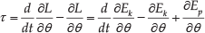
Based on the Lagrange function L, the dynamics equation of the system is:

τ = \frac{d}{d t} \frac{\partial L}{\partial θ} - \frac{\partial L}{\partial θ} = \frac{d}{d t} \frac{\partial E_{k}}{\partial θ} - \frac{\partial E_{k}}{\partial θ} + \frac{\partial E_{p}}{\partial θ}

(7)

3. Sliding mode control

Sliding mode control is a discontinuous control method. When a system vibrates with small amplitude and a high frequency based on a predetermined trajectory, this process is referred to as the sliding mode movement.

The parameters of the sliding mode controller have nothing to do with system parameters and disturbance. Therefore, the characteristics of sliding mode control are high response speed, better robustness, etc. However, the disadvantage of the sliding mode controller is the presence of chattering. Therefore, sliding movement is very difficult to keep balanced when the terminal trajectory of the tool reaches the surface of the sliding mode.

When the cylinder head of the motorcycle is polished by industrial robot ER50-C20, the sliding mode surface for the polished surface will be designed based on operation requirements and workers' experience.

3.1. Design of the sliding surface and the movement of variable structure control using the sliding mode

The movement of variable structure control when using the sliding mode includes two motion states: normal motion and sliding mode state. The sliding control can force the terminal tool to polish the workpiece on the sliding surface, which is designed according to the required polishing surface. According to the characteristics of the sliding mode control, it can be classified as several types of motion states. First, the sliding mode selects a sliding surface, then the tool reaches the sliding surface from any initial state within a limited time. This process is called the reaching phase. When the trajectory of the tool reaches the sliding surface, it stays on the sliding surface and moves around the sliding surface. This process is called the sliding mode. These processes are together referred to as the sliding mode control. However, a stable error can occur as the result of buffeting. Thus, the design of the sliding surface is extremely important.

The linear system can be shown as follows:

\dot{x} = A x + b u

where, ${\dot{x}}_{i} = x_{i + 1}, i - 1, …, n - 1.$

The sliding surface can be obtained thus:

s (x) = C^{T} x = \sum_{i = 1}^{n} c_{i} x_{i}

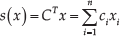
where x is the state vector, $C = {[c_{1}, c_{2}, …, c_{n - 1}, 1]}^{T}$

$c_{1} + c_{2} p + … + c_{n - 1} p^{n - 2} + p^{n - 1}$ should be Hurwitz polynomial.

The state vectors of this paper are $e = θ_{d} - θ$ and $\dot{e} = {\dot{θ}}_{d} - \dot{θ}$ ; therefore, the sliding surface is chosen based on the polishing surface and the sliding function is given by:

s = c e + \dot{e}

(8)

where

s= sliding function.

c= the coefficient of the sliding mode and its value is decided by the machining material. In general, c>0.

e = the error of joint angular displacement.

Depending on the requirements of polishing, a flow chart can be designed as shown in Fig.3. The error of angular displacement of joint 6 is regarded as the input e.

Figure 3.

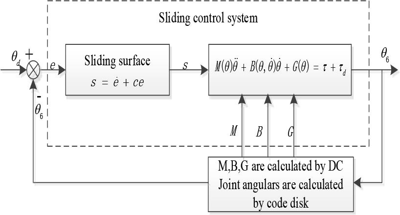
Sliding mode control system structure

During the working process of industrial robot ER50-C20, the external disturbance is unknown. Buffeting will appear and therefore, the system error will be large. When the burr of the workpiece is polished by the tool, the cutting force is decided by the workpiece material. The amounts of feed and feed rate are given. According to the study of actual machining, the error that comes from buffeting and cutting force is the largest. In order to ensure that the actual machining trajectory and artificial teaching trajectory are close to each other, this type of error should be minimized in order to meet machining requirements. The function f(x) represents the sum of two types of errors. If the value of function f(x) is designed to be the minimum, the machining quality of the workpiece will be improved. The RBF network, which has been introduced in this paper, can solve this problem.

4. RBF neural network based sliding mode control scheme

In order to enhance the accuracy of tracking the position of the tool and to reduce the error of conventional sliding mode control, the RBF network control is introduced.

4.1. RBF neural network

The radial basis function neural network (RBFNN) is a type of feedforward neural network. To date, it has shown the best approximation performance among such networks, as well as global optimization capability.

The chattering phenomenon can be alleviated by using RBFNN to adjust the gain of the sliding mode controller. The principle of RBF is to use a radical base as the base of the hidden layer unit to form a hidden layer space. The relationship between the input layer and hidden layer is nonlinear. However, the relationship between the hidden layer and output is linear. The input data can be transferred from a low-dimensional mode to a high dimensional mode using this relationship. At the same time, the RBFNN can change the linearity inseparable problem in the low-dimensional space into a separable problem in the high-dimensional space. The RBFNN, therefore, can approximate any nonlinear function.

The terminal trajectory of the robot is presented in this paper. The joint error and change rate of joint error are regarded as inputs, while output will be calculated by RBFNN based on the sliding mode control. The radial basis vector is $H = {[h_{1}, h_{2}, … h_{6}]}^{T}$ and the weight vector of the network is $W = {[w_{1}, w_{2}, … w_{6}]}^{T}$ . The output is given by:

y (k) = W * H = \sum_{i = 1}^{6} w_{i} h_{i}

(9)

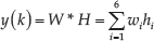
The number of sample points on the trajectory is numerous and it is important to choose proper points to describe the machining process. These points should be convergence points. According to the work conditions and workers' experience, the Gauss basis function is a better option for application in this paper.

h_{i} = \exp (- \frac{{‖ X - c_{i} ‖}^{2}}{2 b_{i}^{2}}), i = 1, 2, …, 6

(10)

f (x) = W^{T} * h (x) + ε

(11)

where

$f (x)$ = external disturbance and uncertainty.

ε = the tracking error of the network.

The i^th centre vector of the neural network is described by $c_{i} = [c_{i 1}, c_{i 2}, … c_{i 6}]$ .

The base width vector of the neural work is described by $B = {[b_{1}, b_{2}, … b_{6}]}^{T}$ .

b_i = the base width parameters of the i^th node.

The input of the neural network is given by:

X = {[e, \dot{e}]}^{T}

(12)

According to workers' experience, a three-layer neural network control strategy is chosen to approximate to output, as shown in Fig.4.

Figure 4.

The structure of the three-layer neural network

This three-layer network structure includes an input layer, hidden layer and output layer. The neurons are used for mathematical operations in the hidden and output layers. The generalization and complexity of the neural network are affected by the number of neurons in the hidden layer. The joint error e and change rate of joint error e_c are regarded as inputs for the input layer, and they are mapped to the hidden layer by a Gauss basis function. The Gauss basic function is linearly mapped to the output layer to obtain the output function.

The dynamics equation is modified by:

\ddot{θ} = M^{- 1} (θ) [τ + τ_{d} - B (θ, \dot{θ}) \dot{θ} - G (θ)]

(13)

\dot{θ} = - s + θ_{d} + c e

(14)

The size and height of the burr and the external disturbance cannot be calculated using a mathematical model; therefore, these uncertainties are described by function f₁:

M \dot{s} = M ({\ddot{θ}}_{d} - \ddot{θ} + c \dot{e}) = - B s - τ - τ_{d} + f_{1}

(15)

Combining Equations (9), (14) and (15), we have:

f_{1} = M ({\ddot{θ}}_{d} + c \dot{e}) + B ({\ddot{θ}}_{d} + c \dot{e}) + G

(16)

The maximum of f₁ should be limited and its value is determined by the manufacturing demand and roughness of standard workpieces.

According to the description in section 3, the error caused by chattering and cutting force is the primary aspects of function f₁. Therefore, it is important to study cutting force.

4.2. The RBFNN-SMC control scheme for the deburring robot system

For the same workpiece, burr size will be different in different locations. Cutting depth is also adjustable based on machining requirements. The artificial teaching trajectory is adjusted based on the specific workpiece. This process is detected by the force and torque sensors, while burr size is detected by the cutting depth. The magnitude of the cutting force depends on the cutting depth; as such, it is necessary to study the relationship between cutting force and cutting depth. Cutting force is proportional to cutting depth [14] and is given by:

F = K \times M R R = K \times (S_{1} + S_{2}) v_{t o o l}

(17)

where

K = the material coefficient of the cylinder head of the motorcycle.

$M R R$ = the amount of material removal from the cylinder head of the motorcycle.

S₁ = the cross sectional area of cutting angle.

S₂ = the cross sectional area of the burr.

$v_{t o o l}$ = the feed rate of the tool.

During the actual machining process, the magnitude of the cutting force is a key parameter for guaranteeing product quality. The size of the burr is uncontrollable and the cutting force is an important aspect of uncertainty. The uncertainty function $f (x)$ is given by:

f (x) = M ({\ddot{θ}}_{d} + c \dot{e}) + B (θ_{d} + c e) + G + F

(18)

As shown in Fig.4, the neural network control strategy can reduce the error caused by chattering and cutting force. The network's working principle is shown in Fig.5. The desired joint angular displacement $θ_{d}$ is obtained after artificial teaching. The angular error e of the sixth joint is defined as the input, which is the difference between the desired angular displacement $θ_{d}$ and actual angular displacement $θ_{6}$ . Once the sliding surface has been chosen, the combination of input e and the sliding surface is the sliding mode function. The sliding mode control is unable to solve the problem alone and the RBFNN is combined with the sliding mode control. The Gauss basic function is also combined with the RBFNN control strategy. Optimal actual joint angular displacement $θ_{6}$ is obtained in the closed RBFNN control system. In Fig.5, the feed rate of tool $v_{t o o l}$ , inertial mass and the gravity torque of the 6^th joint are calculated.

Figure 5.

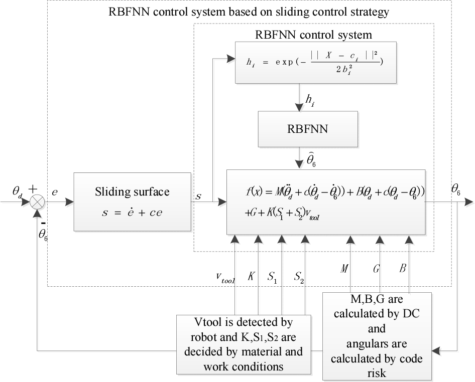
The control structure of RBFNN based sliding mode scheme

5. Simulation analysis

The methods described in this paper were tested in simulations for the ER50-C20 robot according to the original values of joint θ = [-0.563rad, −0.183rad, −0.656rad, −0.996rad, 1.283rad, 0.996rad] and the final values of joint $θ^{'}$ = [-0.507rad −0.715rad −0.353rad −1.114rad 1.319rad 1.183rad]. The robot's end-effector moved from point A (1322mm, −670mm, 1035mm) to point B (1363mm, 120mm, 1265mm) in Cartesian space and 100 points were sampled between A and B. The sampling time was 20 seconds and sampling interval was 0.2 seconds. The size of the burr was measured by Vernier calliper. The height of the burr at point A was roughly 0.5mm, i.e., h=0.5mm. The cutting depth at point A was roughly 0.3mm, i.e., h1=0.3mm. According to the description in section 4.2, cutting force could then be calculated. In this paper, parameters were chosen based on machining requirements. The input of RBFNN is $X = {[e, \dot{e}]}^{T}$ and the terminal trajectory is given by $θ_{d 6} = 1 + 0.1 \sin (t)$ .

The end-effector trajectory was determined by the artificial teaching method, as shown in Fig. 6. The figure also shows the end-effector's three dimensional trajectory.

Figure 6.

Orientation of the end-effector

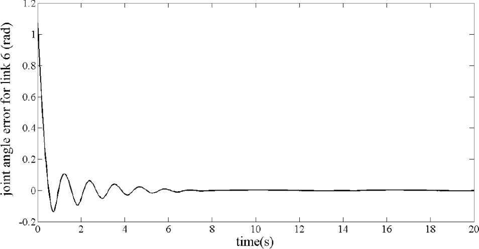
The performance of the RBFNN based sliding model control was shown to be better than the conventional sliding mode control. During the machining process, the conventional sliding mode control requires a long setting time, roughly seven seconds, as shown in Fig. 7. However, the RBFNN sliding mode control has a short setting time of three seconds, as shown in Fig. 8. The red solid line represents the ideal terminal angle, while the black dotted line represents the actual terminal angle during the machining process. Fig.9 shows the error curve based on the sliding mode and Fig.10 shows the error curve based on the RBFNN sliding mode. The maximum error value of the terminal joint angle was roughly 0.25rad in the equilibrium position, as shown in Fig.9. The maximum error value of the terminal joint angle was roughly 0.02rad in the equilibrium position, as shown in Fig.10. Therefore, the error of the RBFNN sliding mode was smaller than for the sliding mode. Compared with the sliding mode method, machining accuracy will be improved by the RBFNN sliding mode control. The simulation indicates that setting time was greatly reduced and the joint angular error was also decreased by the RBFNN sliding mode control.

Figure 7.

Terminal joint angle of robot based on sliding mode control

Figure 8.

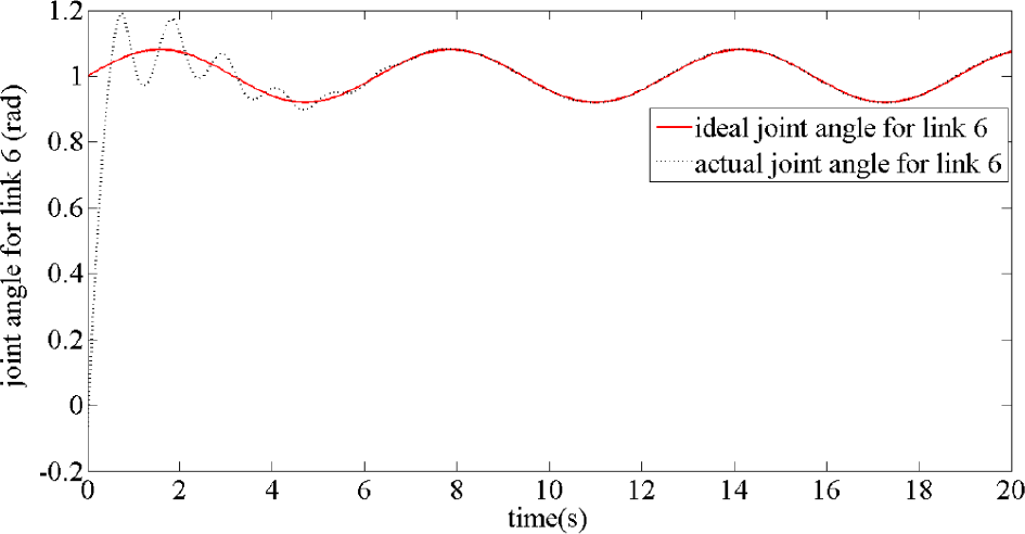
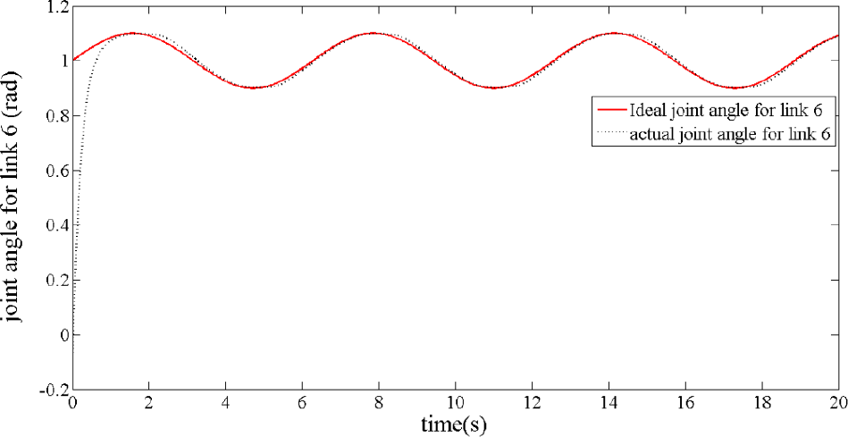
Terminal joint angle of robot based on RBFNN sliding mode control

Figure 9.

Terminal joint angle error of robot based on sliding mode control

Figure 10.

Terminal joint angle error of robot based on RBF sliding mode control

In Fig.11, which represents the conventional sliding mode control, the red solid line represents the ideal terminal joint angular velocity, while the black dotted line represents the actual terminal joint angular velocity during the machining process. Between one second and four seconds, the terminal joint angular velocity is large and its change range veers between −0.7rad/s and 0.5rad/s. This means that velocity is not uniform and the buffeting phenomenon appears, causing the smoothness of the surface to be broken. However, the terminal joint angular velocity is almost approximate to the ideal joint angular velocity in Fig.12, which represents RBFNN sliding mode control. Therefore, the smoothness of the surface based on RBFNN sliding mode control is better than that based on sliding mode control. The setting time is roughly seven seconds in Fig.13; however, setting time is roughly two seconds in Fig.14. Therefore, the RBFNN sliding mode controller has a shorter setting time than the traditional sliding mode controller. The quality of the workpiece will therefore be improved by adopting the RBFNN sliding mode controller.

Figure 11.

Terminal joint angular velocity of robot based on sliding mode control

Figure 12.

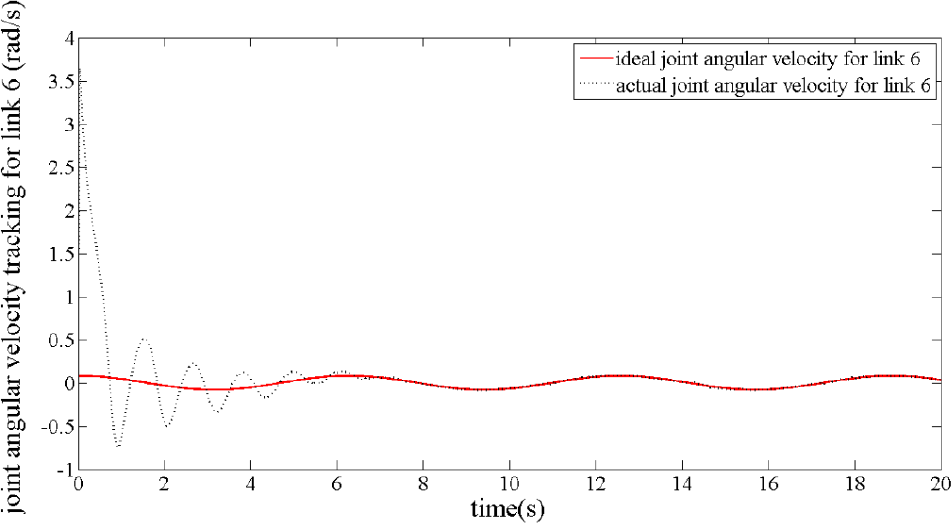
Terminal joint angular velocity of robot based on RBF sliding mode control

Figure 13.

Terminal joint angular velocity error of robot based on sliding mode control

Figure 14.

Terminal joint angular velocity error of robot based on RBF sliding mode control

As shown in Fig.15, which represents the conventional sliding mode control, the red solid line represents ideal uncertainty factors, while the black dotted line presents the actual uncertainty factors during the machining process. The disturbance factor is large prior to seven seconds. However, the disturbance factor is small prior to five seconds in Fig.16. Fig.17 represent the sliding mode control and Fig.18 represent the RBFNN sliding mode control. As shown in Fig.17, which represents the conventional sliding mode control, the maximum error is almost 60N*mm and the average error is almost 25N*mm during setting time. As shown in Fig.18, the maximum error is about 20N*mm during setting time. Compared to the conventional sliding mode controller, the disturbance factors have been reduced by adopting the RBFNN sliding mode controller. Therefore, the performance of the RBFNN sliding model control is better than the conventional sliding mode control.

Figure 15.

Uncertainty factors based on sliding mode control

Figure 16.

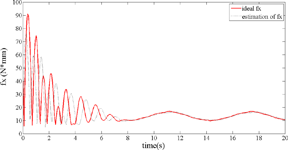
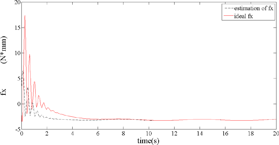
Uncertainty factors based on RBF sliding mode control

Figure 17.

Uncertainty factors error based on sliding mode control

Figure 18.

Uncertainty factors error based on RBF sliding mode control

6. Conclusion

A RBFNN-SMC method was implemented to control the joint movements of a deburring robot manipulator. A dynamic model was established and robustness and accurate position tracking was achieved. The RBFNN-SMC method integrates the properties of SMC robust control, which learns uncertain control actions and relaxes the requirements of the system's accurate model. The RBFNN-SMC method for the deburring robot was developed without the requirements for strict constraints, an accurate model and exact parameters. The proposed RBFNN-SMC scheme was evidenced from comparisons with previous control schemes.

The simulation results show that the RBFNN sliding mode controller can satisfactorily meet deburring processing requirements. Compared to the conventional sliding mode controller, the RBFNN sliding mode controller can guarantee the stability of the machining processing and reduce potential uncertainties.

Footnotes

7. Acknowledgements

This work was supported by the Youth Science Fund Project NO.61305116of the National Natural Science Foundation and Major Science and Technology Projects of the Chongqing Robot Industry No.cstc2013jcsf-zdzxqqX0005.

References

Abanovic

Variable Structure Systems with Sliding Modes in Motion Control – A Survey[J]. IEEE Transactions on Industrial Informatics, 2011, 7(2):212–223.

Taheri

Case

Richer

Force and Stiffness Backstepping-Sliding Mode Controller for Pneumatic Cylinders[J]. IEEE/ASME Transactions on Mechatronics, 2014, 19(6):1799–1809.

Yang

Wang

Q L

Sliding mode variable structure control theory: A survey[C]//2012 31st Chinese Control Conference (CCC), 2012:3197–3202.

Sharkawy

A. B.

Salman

S. A.

, “An adaptive fuzzy sliding mode control scheme for robotic systems”, Intelligent control and automation, pp. 299–309, 2011.

Rubagotti

Estrada

Castanos . Integral Sliding Mode Control for Nonlinear Systems With Matched and Unmatched Perturbations[J]. IEEE Transactions on Automatic Control, 2011, 56(11): 2699–2704.

Mahmoodabadi

M J

Taherkhorsandi

Bagheri

Optimal Robust Sliding Mode Tracking Control of a Biped Robot based on Ingenious Multi-objective PSO[J]. Neurocomputing, 2014, 124(2):194–209.

Topalov

A V

Kaynak

Shakev

N G

. Neural network identification, predictive modeling and control with a sliding mode learning mechanism: an application to the robotic manipulators[C]//First International IEEE Symposium “Intelligent Systems”, Proceedings. IEEE, 2002:102–107.

Chaouch

D E

Ahmed-Foitih

Khelfi

M F

. A sliding mode based control of 2dof robot manipulator using neural network[C]//2012 6th International Conference on Sciences of Electronics, Technologies of Information and Telecommunications (SETIT), IEEE, 2012:906–911.

Kayacan

Ramon . Adaptive Neuro-Fuzzy Control of a Spherical Rolling Robot Using Sliding-Mode-Control-Theory-Based Online Learning Algorithm.[J]. IEEE Transactions on Cybernetics, 2013, 43(1):170–179.

10.

Engeberg

E D

Meek

S G

. Adaptive Sliding Mode Control for Prosthetic Hands to Simultaneously Prevent Slip and Minimize Deformation of Grasped Objects[J]. IEEE Transactions on Mechatronics, 2013, 18(1):376–385.

11.

Meng

Zhang

Gao . Adaptive Sliding Mode Fault-Tolerant Control of the Uncertain Stewart Platform Based on Offline Multibody Dynamics[J]. IEEE Transactions on Mechatronics, 2014, 19:882–894.

12.

Guo

Woo

P Y

. An adaptive fuzzy sliding mode controller for robotic manipulators[J]. IEEE Transactions on Systems Man & Cybernetics Part A Systems & Humans, 2003, 33(2):149–159.

13.

Han

S I

Lee

J M

. Precise Positioning of Nonsmooth Dynamic Systems Using Fuzzy Wavelet Echo State Networks and Dynamic Surface Sliding Mode Control[J]. IEEE Transactions on Industrial Electronics, 2013, 60(11):5124–5136.

14.

Zhang

M J

Chu

Z Z

. Adaptive sliding mode control based on local recurrent neural networks for underwater robot[J]. Ocean Engineering, 2012, 45(2):56–62.

15.

Wai

R J

Muthusamy

Fuzzy-neural-network inherited sliding-mode control for robot manipulator including actuator dynamics[J]. IEEE Transactions on Neural Networks & Learning Systems, 2013, 24(2):274–287.

16.

Siradjuddin

Behera

McGinnity . Image-Based Visual Servoing of a 7-DOF Robot Manipulator Using an Adaptive Distributed Fuzzy PD Controller[J]. IEEE/ASME Transactions on Mechatronics, 2014, 19(2):512–523.

17.

Chen

C S

. Robust Self-Organizing Neural-Fuzzy Control With Uncertainty Observer for MIMO Nonlinear Systems[J]. IEEE Transactions on Fuzzy Systems, 2011, 19(4):694–706.

18.

Lian

R J

. Adaptive Self-Organizing Fuzzy Sliding-Mode Radial Basis-Function Neural-Network Controller for Robotic Systems[J]. IEEE Transactions on Industrial Electronics, 2014, 61(3): 1493–1503.

19.

Sun

Pei

Pan . Neural network-based sliding mode adaptive control for robot manipulators[J]. Neurocomputing, 2011, 74(1415):2377–2384.

20.

Peng

Bai

Gong . Modeling and robust backstepping sliding mode control with Adaptive RBFNN for a novel coaxial eight-rotor UAV[J]. IEEE/CAA Journal of Automatica Sinica, 2015, 2(1): 56–64.

21.

Jin

Chang

P H

Jin . Stability Guaranteed Time-Delay Control of Manipulators Using Nonlinear Damping and Terminal Sliding Mode[J]. IEEE Transactions on Industrial Electronics, 2013, 60(8):3304–3317.

22.

Capisani

L M

Ferrara

Trajectory Planning and Second-Order Sliding Mode Motion/Interaction Control for Robot Manipulators in Unknown Environments[J]. IEEE Transactions on Industrial Electronics, 2012, 59(8):3189–3198.

23.

Wang

Chai

Zhai

Neural-Network-Based Terminal Sliding-Mode Control of Robotic Manipulators Including Actuator Dynamics[J]. IEEE Transactions on Industrial Electronics, 2009, 56(9):3296–3304.

24.

Kikuuwe

A Sliding-Mode-Like Position Controller For Admittance Control With Bounded Actuator Force[J]. IEEE/ASME Transactions on Mechatronics, 2014, 19(5):1489–1500.

25.

Mickael

Kourosh

Mohammad

M F

. Design of fuzzy controller for robot manipulators using bacterial foraging optimization algorithm [J]. Journal of intelligent learning systems and applications, 2012, 4:53–58.

26.

Salem

Saeed

M B

. Stable adaptive neural control of a robot arm [J]. Intelligent control and automation, 2012,3:140–145.

27.

Meza

J L

Soto

Llama

M A

. Fuzzy self-tuning PID semiglobal regulator for robot manipulators [J]. IEEE Transactions on industrial electronics, 2012, 59(6): 2709–2717.

28.

Indrazno

Laxmidhar

McGinnity

T M

Sonya

Image-based visual servoing of a 7-DOF robot manipulator using an adaptive distributed fuzzy PD controller [J]. IEEE Transactions on mechatronics, 2014, 19(2): 512–523.

29.

Liu

Tang

Zeng

Z Y

. Feature selection based on dependency margin [J]. IEEE Transactions on CYBERNETICS, 2015,45(6): 1209–1221.

30.

Liu

Huang

W L

Jiang

Y L

Zeng

Z Y

. Quick attribute reduct algorithm for neighborhood rough set model [J]. Information Science, 2014, 271: 65–81.

31.

Liu

Xiong

Robust and Accurate Multiple-camera Pose Estimation Toward Robotic Applications. International Journal of Advanced Robotic Systems, 2014,11:1–13.

32.

Jiang

Y L

Y X

Liu

Performance evaluation of feature detection and matching in stereo visual odometry. Neurocomputing, 2013, 120: pp. 380–390.

A Sliding Mode Control-Based on a RBF Neural Network for Deburring Industry Robotic Systems

Abstract

Keywords

1. Introduction

2. Dynamic model of a 6-DOF deburring robot

3. Sliding mode control

3.1. Design of the sliding surface and the movement of variable structure control using the sliding mode

4. RBF neural network based sliding mode control scheme

4.1. RBF neural network

4.2. The RBFNN-SMC control scheme for the deburring robot system

5. Simulation analysis

6. Conclusion

Footnotes

7. Acknowledgements

References