
Abstract
A three-dimensional coverage path-planning algorithm is proposed for discrete harvesting machines. Although prior research has developed methods for coverage planning in continuous-crop fields, no such algorithm has been developed for discrete crops such as trees. The problem is formulated as a graph traversal problem and solved using graph techniques. Paths to facilitate autonomous operation are generated. A case study is formed around the novel tree-to-tree felling system developed by the University of Canterbury and Scion. This machine is being developed to manoeuvre through New Zealand's plantation forest to fell Pinus radiata trees on steep (≤ 45°) terrain. Algorithm performance is evaluated in 14 commercial plantation forests. Results indicate that a mean coverage of 84.43% was achieved.
Keywords
Introduction
New Zealand's forest industry is the country's third largest export earner, contributing 2.9% of the gross domestic product [1]. Additionally, in 2010, New Zealand was ranked in the top 20 of global wood suppliers and is forecast to be in the top five by 2025. The first and second biggest export earners are also both from primary industries: “Milk powder, butter, and cheese” and “meat and edible offal”, respectively [2]. Increasing global and domestic demand has led to a large growth in use of robotic platforms in the primary industry. Other factors, such as smaller rural labour forces and sustainability, have also had an influence. The McKinsey Global Institute identified advanced robotics as a potentially disruptive technology due to its capacity to completely change the status quo [3]. Robotics in agriculture have the potential to decrease the vulnerability of workers in dangerous working conditions and increase the efficiency of time, materials and resources through better utilization and planning. Primary industries have already seen a wealth of promising robotic harvesting platforms but, despite success in other areas, only limited developments have occurred for the forest industry. In 2012, it was reported by Raymond [4] that 77% of tree felling in New Zealand is performed manually using chainsaws. The steep terrain of the country's plantation forests limits the utilization of machines. The forest industry is the country's most injury- and fatality-prone; the high rate of manual felling is a leading contributor to this statistic. Therein lies the motivation to develop a tree-felling machine that can work on any terrain without the need for an operator nearby. As yet, to the authors’ knowledge, there exists no machine that can move from tree to tree without touching the ground in order to harvest trees.
Related Work
A robotic arm system has been reported by Foglia and Reina [5] for the purpose of harvesting the vegetable radicchio. This system used computer vision from a monocular camera to localize the target. A linkage system was developed to cut and retrieve the vegetable from its growing position in the soil. The system was a static arm designed to be mounted to a moving tractor, with the ability to harvest one radicchio plant every seven seconds. Route planning was limited to the nearest neighbour, approached in the row selected by the operator. Due to a labour shortage of seasonal workers in Japan, a cherry-harvesting robot was developed by Tanigaki et al. [6]. By combing the data from two pulsed-laser beams, the positions of cherries were calculated. Analysis of the data returned by the laser beam classified cherries and obstacles according to the components of the reflected light spectrum. Further agricultural developments include devices for cucumbers [7], apples [8] and strawberries [9]. From the literature previously cited, it has been shown that robotic harvesting is more than just a possibility; despite this, only limited developments have occurred in the forestry industry. Tarn and Xu [10] describe a small, agile tree-climbing robot capable of manoeuvring on a tree through the use of two grippers connected by a flexible body. The robot implements an autonomous climbing algorithm to explore the tree with goals such as animal observation or tree maintenance. A tree-pruning device developed by Soni et al. [11] is positioned on a tree by a human operator. The device encircles the tree and uses wheels to propel itself along the tree trunk. A five degree of freedom arm is mounted onto the platform that executes the pruning task. Research interest in forest robotics has focused on pruning measurement and exploration rather than on felling.
Work to date on coverage path planning has considered applications involving machines such as tractors for field-based operations. The issue of spreading seed on fields using tractors is addressed by Jin and Tang [12] and Hameed [13] covered other generic field maintenance tasks such as fertilizing. Hameed developed a planning approach that extends beyond flat fields to 3D terrain. This implements an energy-consumption model of the machine in order to plan the optimal driving direction. This approach minimizes the direct energy needed by the vehicle when it is travelling in parallel paths along the field. Jin and Tang showed how elevation models can be used to form analytical models by identifying subregions in the terrain. These subregions were individually optimized according to their unique features, as opposed to adopting a single solution for all terrain approaches. Once a path was found through the area, parallel work paths were formed by offsetting the curve to the edges of the workspace. These planning approaches address the issue of covering a large, three-dimensional field with a tractor-type vehicle while seeking to maximize the area covered. The objective crops in previous schemes are in a highly structured environment consisting of rows or parallel paths that have simple geometries. The tasks of the machinery are generally ‘area coverage’ operations, for instance, that of spraying a field.
Bochtis et al. [14] generalized the planning of orchard operations to the form of a graph problem. In their case, operations need to be done row-wise. Such tasks include mowing, spraying and harvesting. Indeed, Bochtis and S⊘rensen [15] show that vehicle routing-problems are a generalized case of the Travelling Salesman Problem. To form the graph, nodes were used to represent the start and end points of each row, and a corresponding matrix of connection costs was generated. Bochtis et al. [16] also extended their approach to field planning for deriving a path for wildlife avoidance that was based upon escape models for the animals. For planning Kang et al. [17] used a machine-learning approach for stochastic node models, and Bao et al. [18] showed how machine learning can be coupled with computer vision and human interaction in planning paths, even in intricate environments. The Depth First Search (DFS) and the Breadth First Search (BFS) are commonly used to traverse graphs, Gleich [19] provides implementations. The BFS operates by first exploring nodes on the same level before investigating their children, whilst the DFS will always explore children before returning to the level above. The differences between the DFS and the BFS come down to the data structure used to store the discoveries: in the DFS it is a stack, whereas the BFS uses a queue [20]. The Travelling Salesman Problem (TSP_NN), following Kirk's [21] implementation, determines the route by always visiting the next closest node until the end node is reached. Fatime, [22], presented a graph-searching algorithm to find the specified length between two nodes. Fatime's approach, however, suffered from having to maintain arrays that grew too large for a computer to store.
In order to manage large commercial forests, operators require many metrics on its performance: using both “traditional data types and remotely sensed data is widely recognized as essential and critical for extensive ‘on-time’ environmental studies and monitoring at the local, regional (landscape), and national levels” [23]. Due to the scale of these operations, accessibility can be an issue; hence, it is common for data to be collected aerially from sources such as satellites, aeroplanes, helicopters and balloons. LiDAR and images at a variety of wavelengths are commonly returned data. Maltamo et al. [24] described many of these applications for airborne LiDAR. Analysis of this data is used to provide the end user with information of “forest area, volume, condition, growth, mortality, removals, trends, and forest health” [25]. LiDAR has been proven effective in estimating the biomass, canopy volume and mean height of large footprint systems by Lim et al. [26], whilst small footprint systems are able to inform the user on the crown width and height of individual trees. Culvenor's work [27] shows how high-resolution imagery can be used to delineate tree crowns. By considering the changes in brightness between the centre and edge of the crown, in the near infrared, red and green bands, container cells are formed. These cells contain the detected canopy and the tree crown's location can be found using a local maxima search.
The novel contribution of this paper is that of solving the two- and three-dimensional coverage route-planning problem for a node-to-node style-harvesting machine. This has applications for a wide variety of field robotics that must visit multiple discrete sites, even outside harvesting such as search and rescue, security and the scientific sampling of interest points. Optimizing visitation to these sites can improve performance in measures such as time, vehicle lifetime and fuel consumption. The current state-of-the-art practice for coverage path planning, as applied to harvesting has been limited to continuous crops such as wheat in large fields. Currently there are no such algorithms for harvesting discrete objects such as trees, to the knowledge of the authors: a lack addressed by this work. Further, a generic partitioning strategy is developed allowing the integration of other planners that were previously impractical for large graphs. A case study is formulated based upon the tree-felling machine developed by Meaclem et al. in [28]. In the study, the application of tree felling is modelled using graph representation and approached via the proposed node-visitation method.
In this paper, the methodology of the proposed algorithm is introduced first. The proposed method is then bench-marked against three other algorithms and results analysed in the discussion. Limitations and future works are identified, before the paper offers concluding remarks.
Tree-to-tree Felling Machine
A quarter-scale, tree-traversing robot has been developed [28]. The design consists of three basic elements: the arms, wrists and grippers. The machine begins locomotion with one gripper fixed to a tree, while the opposite gripper (end-effector) is free to move. Locomotion is achieved by turning the robot toward the next tree using the wrist motors, and then reaching out towards the next tree through a coordinated movement of actuators in the arm. Upon reaching the next tree, the end-effector closes to secure its grip whereupon the initial actuator is released. By repeated cycles of grab and release, the machine traverses the forest (see Figure 1).
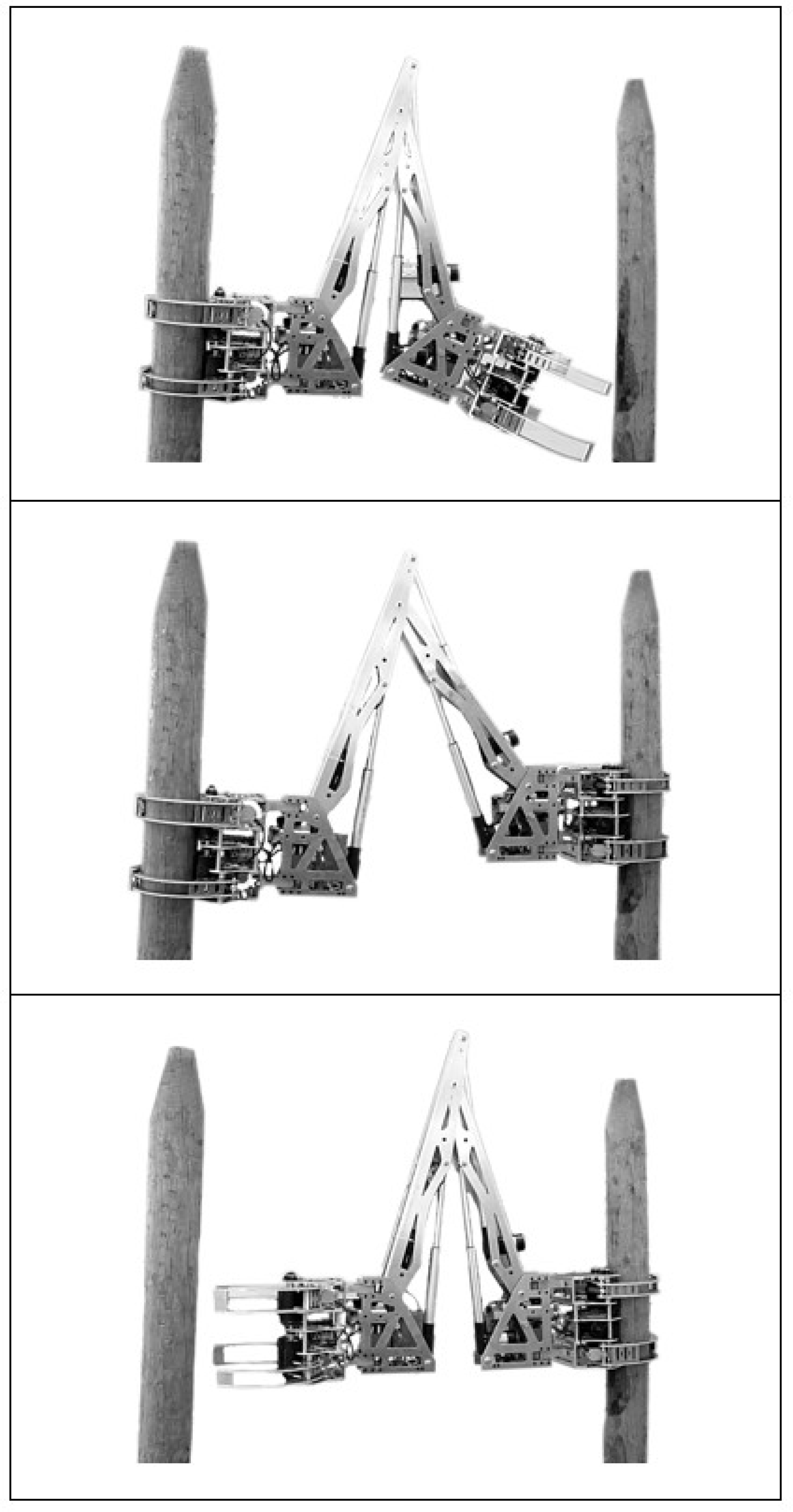
Traversal of the robot. Top: starting position. Centre: attached to both trees. Bottom: release of initial tree. [28]
A chainsaw mechanism mounted below the gripper facilitates the tree felling. The felling process is conducted whilst the machine is attached to trees at both ends in order to provide stability. The underslung chainsaw advances into the trunk according to a felling policy based upon sensory data and user input regarding the tree. Towards the end of the cut, when the tree is detected as being close to falling, the gripper is released. Cutting continues but, at this stage, the robot is now detached from the tree, which allows it to fall. The cutting policy designs the cuts so that the tree falls away from the machine.
For many applications in harvesting, the former coverage cases can be an ill-fitting abstraction of the problem. Where the object to be harvested can be considered as discrete (for example, radicchios and pine trees) as opposed to continuous (maize or sugarcane), then a more fitting abstraction might be that of a node-visitation problem. Consider a commercial plantation forest on New Zealand's rough, steep terrain; despite the best intentions of the forest's managers, trees that are planted in rows often develop over their 30-year lifespan to adopt irregular positions and poses due to a variety of environmental factors. In this and other such cases, each element of the crop can be considered a node, and a path between nodes can be considered an edge. The methodology considers the approach taken towards coverage path planning for the purpose of discrete harvesting. Nodes can only be visited once, since they are removed upon harvesting. After the node has been visited, it cannot be used as a ‘stepping stone’ to traverse to other nodes.
The methodology can be broken down into four constituent parts, namely: A. edge identification, where inter-tree path options are identified; B. graph representation, where a graph model is created; C. partitioning, to reduce the computational complexity and D. partitioned space path planning using k-means (KPSPP), the path-planning operation.
Edge Identification
The input to the algorithm is the data collected from the forest inventory, including the latitude, longitude and altitude for each of the n trees. These tree data might be obtained, for example, by using aerial LiDAR or terrestrial GPS. This paper uses provided forest maps which have been generated by finding the crown location and inferring the trunk location at ground level from Pont el al [29]. From these known tree locations, the algorithm must derive the graph structure. The graph-structure abstraction sets the basis for the coverage path. Whilst nodes are readily determined from the tree-location data by the one-to-one relationship of trees to nodes, graph edges need to be defined.
In the forest, there are no predefined paths between trees; therefore, inter-tree paths are defined as the edges of the triangles generated in the Delaunay triangulation. By using the Delaunay triangulation, nodes are connected in the nearest-neighbour fashion. The triangulation also contains the minimum spanning tree and convex hull of the set. Points on the convex hull are the most likely starting points for a harvesting machine due to their convenient location on the periphery of the harvesting area. From the latitude and longitude of each node, the triangulation is computed. By decomposing the resultant triangles into their edges, ε paths between nodes are established.
The Delaunay triangulation determines edges as shown in Figure 2. Tree locations, shown as circles, are fed into the triangulation algorithm. All edges from the triangulation are shown as dashed lines. Due to the limited workspace of the machine, however, not all of these edges can be traversed. A filtering step removes edges too long or too short for the machine based upon the 3D Euclidian distance for each edge. The solid lines indicate the traversable paths: these are the paths used in the planning process. These solid lines form the set of edges ε.

Paths resulting from applying the Delaunay triangulation: dashed lines indicate all paths, solid lines indicate traversable paths and circles indicate tree locations. Actual coordinates are abstracted due to commercial sensitivity.
To form an efficient data structure to contain the graph connectivity and edge costs, an adjacency matrix α is formed as defined by Equation 1. The edge, ε k , joins two nodes, P i to P j . Each element in the adjacency matrix represents the cost C(ε k ) of travelling along the edge.

‘Relevant’ elements represent traversable edges that have non-zero values. Similarly, zero valued elements are defined as ‘irrelevant’ due to their having a non-traversable property. If the ratio of relevant to irrelevant elements is considered small, then the matrix is said to be sparse. Tewarson [30] indicates that, in practice, if the matrix has in the order of n non-zero elements, for large n, it is considered sparse.
It is inefficient to store the edge costs of a sparsely connected graph in an n by n matrix. An alternative is to use the sparse class of matrices that Matlab offers. MathWorks [26] give an example: Consider the identity matrix for n=10,000. In the standard matrix format, this would require provision for 100 million values. If double precision floating-point numbers are used, this would occupy 800 Mb. In sparse format, this matrix would require approximately 0.24 Mb. In order to use the sparse matrix representation in Matlab efficiently, zero must be used as the edge cost for non-existent edges rather than infinity. This is because sparse matrices only store the values of non-zero elements rather than every element in standard matrices — leading to significant size reduction for large, low-density matrices. Figure 3 shows how the sizes of both matrix-forms change with sample size.
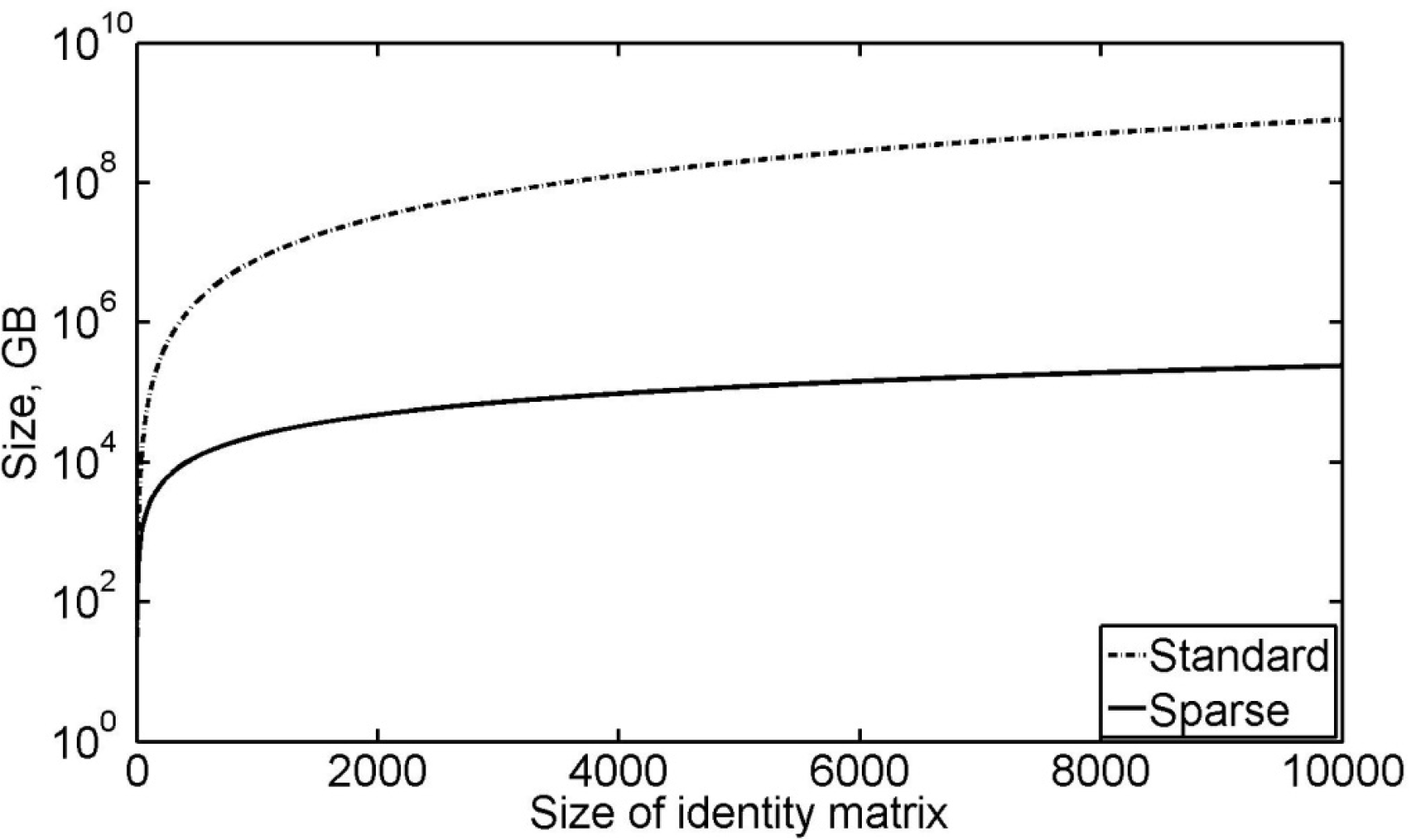
Comparison of the storage size of identity matrices in standard and sparse forms

Matrix size increases exponentially with the number of nodes
The target machine can traverse any edge in either direction; therefore, graph edges are bidirectional. This leads to an adjacency matrix that is symmetrical along the direction of its main diagonal (α i,j = α j,i ). Due to this symmetry, the upper triangular half of the matrix is sufficient to fully define α. The full matrix is formed by an OR operation between the complete upper half and its transposition: α = OR(β, β T ). Although the full matrix can be easily computed, the storage size of the matrix can be halved at this point by using only the upper triangular area.
In the case of harvesting, nodes can be visited exactly once and so the ideal case occurs when all nodes are visited. For n nodes, the longest path has length n. The maximum number of complete paths through the nodes is known a priori, as given by the permutations. Therefore, for n nodes there are no more than n! complete routes. This does not include the partial coverage paths that do not visit every node. A matrix used to store routes through the graph would have dimensions of (n!, n), or larger if partial coverage routes are included. The storage size of this matrix exponentially increases with n and is therefore impractical to maintain, even for small n. The amount of storage required is given by Equation 2 when storing 64-bit numbers.

The rapid growth in size is demonstrated in Figure 4, where at n=11, for example, 3.3 GB of storage is required. For this reason, it is necessary to partition the dataset so that no more than μ nodes are planned in any one set.
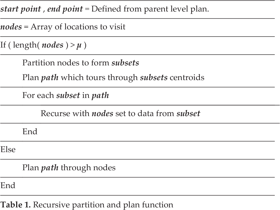
A recursive partitioning strategy is developed. This method reduces the memory requirements of the algorithm by planning only subsets of the total problem and appending the subgroup path to the global path in order to form the global solution. Table 1 describes the algorithm used.
Groups of nodes exceeding μ members must be partitioned to form smaller subsets. Figure 5 illustrates an example forest with 31 trees and a maximum planning capacity, μ, of four. Initially, the forest has 31 trees, a value that exceeds μ. The group is partitioned, therefore, into μ subsets (indicated as yellow, green, blue and red) to form the first level of recursion. The yellow, green, blue and red subgroups contain nine, seven, nine and seven nodes, respectively. This partition of four subsets can now be planned to obtain the order in which they will be traversed; the order obtained might be yellow, green, blue then red. As each subgroup contains more than μ members, they must in turn be partitioned in order to complete the plan in a finer resolution. The yellow subset, containing nine nodes, is divided into three subsets, with yellow, blue and green forming the second level of recursion. As this subset contains fewer than μ members, the path can be planned, resulting in the order yellow, green then blue. At the third level of recursion, each subset now contains fewer than μ members, and so the path through these trees can be obtained directly. Therefore, the path through the trees of the yellow (level one) subset is discovered and forms the beginning of the global path. The algorithm now returns to level one and continues to the next subset according to the plan (green). Again, the algorithm recurses to find the route. Once the route through the trees is achieved for this subset, it is appended to the global path. This repeats for the remaining level-one subsets (blue and red) until the endpoint is reached.
Recursive partition and plan function

The first three levels of recursion for the example of μ = 4
The partitioning of a group is created using the k-means algorithm. Due to the limitation of the number of nodes, it is not possible to create more than μ subsets at any level. The algorithm starts by randomly assigning each data point to one of the μ groups. Nodes are reassigned iteratively to groups so as to minimize the cost of the grouping. The cost is based upon the squared Euclidean distance. Once the cost does not change significantly from iteration to iteration, a local minima has been found and the grouping is complete.
The adjacency matrix summarizing the graph connectivity for any level can be quickly reformed from the global adjacency matrix that was computed initially. The path costs for edges not beginning in the current set are set to zero, the ‘ignore’ case, whilst the edges not finishing in the next set are also set to zero.


In this work, it is assumed that the number of nodes visited is of a higher priority than the cost of the route — the longest route(s) will always be chosen, where options exist the lowest-cost route will be chosen, given that the application is harvesting. Applications of existing algorithms that are limited computationally by the graph size are able to be implemented through the partitioning approach developed.
At the planning stage, start and end points are already defined. The human operator specifies the two points at which the harvesting should start and finish for the set as a whole. In the case of an intermediate set, a point that has connectivity outside of the set to the following subgroup is selected as the end point. The start node for intermediate sets is determined by choosing the point in the next set with the minimum Euclidian distance. The planning component of the algorithm is listed in Table 2. Paths are explored in parallel as and when they are discovered. Starting from the initial node, the adjacency matrix is inspected for edges connecting the current node to others. For each edge that leads to an unvisited node, the previous path is duplicated and the next node is appended to create a new path. This repeats until either the target end point has been reached or there are no nodes left to visit. The latter case occurs when there are no edges connecting the current node to an unvisited node. Routes that do not reach the end point are excluded from further analysis. This returns all possible paths in the set between the start and end points. As all the paths have varied lengths, only the maximal length path is chosen. If there are multiple paths with the same coverage, the algorithm selects the one with the minimal cost according to the sum of the edge costs as defined by the heuristics.
Node planning algorithm

Node planning algorithm
Graph Formation
In the case of Figure 2, the Delaunay triangulation was computed for a set of 486 nodes. This generated 2,952 distinct edges. Filtering edges due to the machine-span limitation reduced the number of edges down to 1,569 edges, 53% of the original quantity. In the data, natural subsets occur due to geography that the machine cannot bridge. Intervention would be required to assist the machine in traversing from one set to another. The natural subsets also help to reduce the planning problem. Initially, this dataset had 486 nodes in one set; after consideration of the geography, there are four naturally enforced subsets of 401, 67, 19 and two nodes each. The natural subsets occurring in Figure 2 are identified in Figure 6.

Identification of natural subsets within the graph of the dataset. The grey area highlights the largest subset with smaller, peripheral sets to the north, west and south.
The occupation of the adjacency matrix for the largest set in Figure 6 is shown in Figure 7. The figure presents the occupied nodes of the adjacency matrix with black squares; white areas represent empty areas. The square matrix has a width of 401 elements and, in this case, contains 1,274 non-zero elements.

Occupation of the adjacency matrix. Black indicates non-zero elements and white indicates zero-valued elements.
To establish a benchmark for the proposed algorithm, two existing graph-traversing methods and a solution to the Travelling Salesman Problem are implemented.
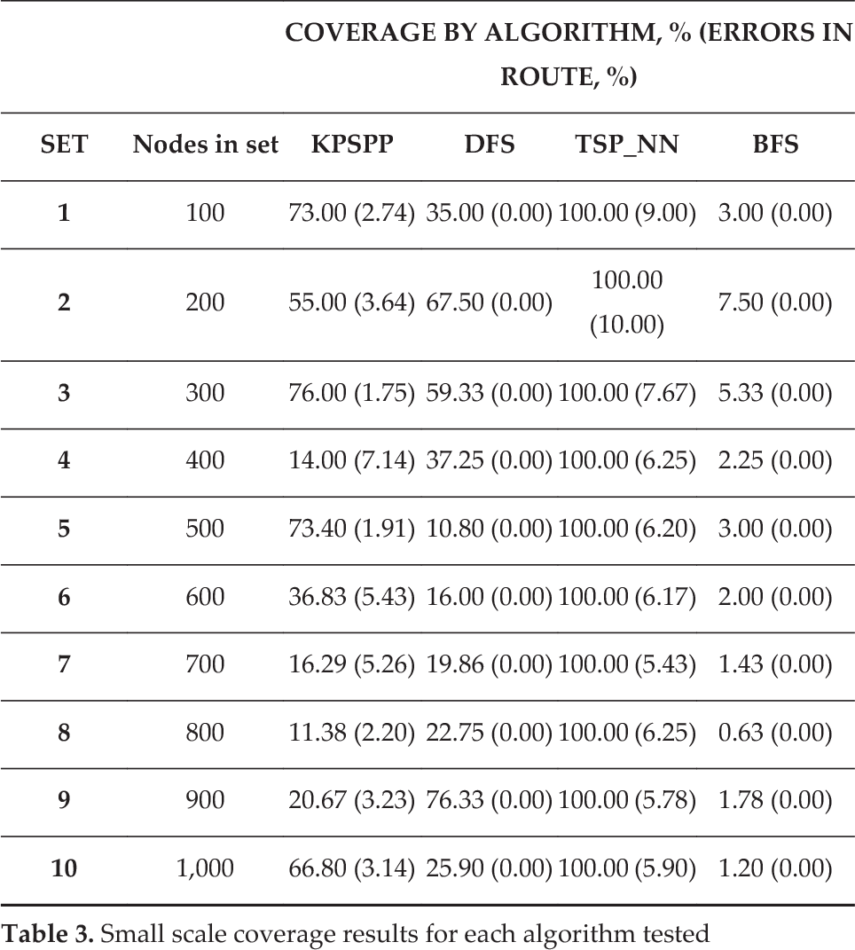
The proposed algorithm was compared with a Depth First Search, a Breadth First Search and a Travelling Salesman Problem implementation based on the nearest-neighbour approach. Algorithms were compared by computing a route between randomly selected start and end points on the convex hull. Evaluations at two different scales were conducted; one investigating the small set performance and a second investigating the large set performance. In the small set tests, algorithms were run on 10 datasets containing 100 to 1,000 trees. In the large-scale tests, the testing of 14 datasets of differing size, containing between 3,500 and 36,000 trees, was performed. In these tests, the datasets comprised measured data from 14 plantation forests and not simulated data. Results for the small-scale testing are listed in Table 3 with summary statistics listed in Table 4. Similarly, for the large-scale testing, results are summarized in Table 5 with summary statistics listed in Table 6.
It was expected from the testing that the DFS and KPSPP would perform similarly, as KPSPP implements a planning approach that is similar to the DFS at its core. As the target application of a BFS is traversing a graph in a short and fast manner, it is expected that this will return paths covering far fewer nodes than the other approaches considered. TSP_NN, being an exhaustive search through the nodes, is expected to return the highest coverage paths but also to take the most time to complete.
Small scale coverage results for each algorithm tested
Small scale coverage results for each algorithm tested
Summary statistics for data presented in Table 3 on small scale testing

Large scale coverage results for each algorithm tested

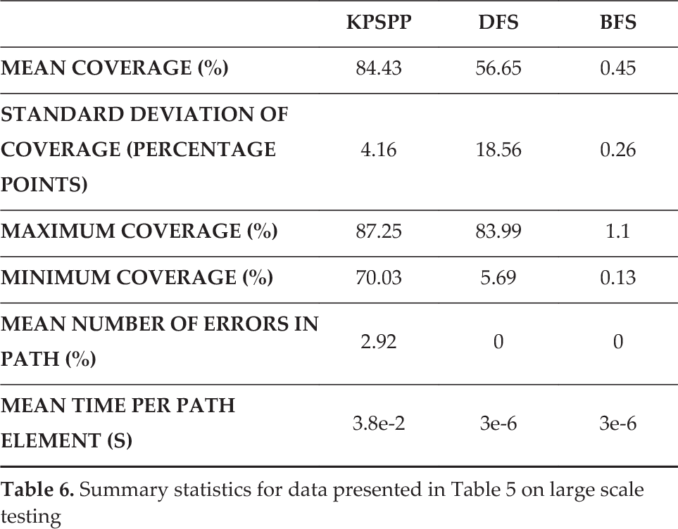
Summary statistics for data presented in Table 5 on large scale testing
The use of sparse matrices is justified by the low occupation of the adjacency matrix, observable in Figure 7. As the matrix contains edge data for 401 nodes and, in this case, contains 1,274 non-zero elements, 0.8% of the available elements contain relevant edge data. In the standard matrix implementation, 99.2% of the space would describe edge costs for non-existent links, which are zero valued. The figure also shows that the data are tightly distributed around the main diagonal, indicating that edges between trees are connected to adjacent trees — as is expected from the Delaunay triangulation definition of edges. Due to the unidirectional edge assumption, the matrix is symmetrical along the main diagonal; this allows for the rapid formation of the entire matrix by using one half to generate the other as A i,j = A j,i .
From the small-scale testing it can be concluded that the DFS and KPSPP performed similarly well with respect to coverage and standard deviation. TSP_NN outperformed KPSPP on the basis of nodes visited (100%); however, it required five times more operator interventions (6.86 compared to 1.36) and took an order of magnitude longer per node. The DFS required no interventions but it outperformed KPSPP at this scale, as it covered approximately the same amount of nodes. The BFS, although requiring no interventions, returned paths that are too short to be considered for coverage planning. At the small scale, the algorithms were ranked as DFS/KPSPP, TSP_NN then BFS (from best to worst).
In the large-scale testing the TSP_NN algorithm could not be tested due to the calculation duration becoming impractically long, in the order of three hours. This shows that the TSP_NN is not practical at this scale. At large scales, the KPSPP algorithm outperformed all others by covering more nodes and in a more reliable manner. KPSPP obtained a mean coverage of 84.43% with a standard deviation of 4.16 – 88% less deviation than the DFS. Although the DFS could produce high coverage paths, it also produced very short paths, resulting in unreliability and, therefore, a large deviation. Again, as for the small-scale testing, the BFS proved to produce paths too short for coverage planning. At the small scale, the algorithms were ranked as KPSPP, DFS, BFS then TSP_NN (from best to worst).
Results show that the DFS algorithm can reliably find a route between the desired points over the range of set sizes. This algorithm returned paths that, on average, visited 56.65% of the available nodes and achieved as high as 83.99% coverage. Although the DFS was able to return paths reliably, it showed large variability in the coverage, which is indicated by a standard deviation of 18.56. A factor affecting the variation is the quantity of outcomes such as paths covering 5.69%, as well as three out of the 14 paths covering less than 50% of the nodes. This variation, the highest of all algorithms considered, decreases its depend-ability in large-scale route planning. As the coverage result is not reliably high, repetition is required to find a suitable path. The DFS does not consider the location of the end point relative to the start point; if the end node is found in a branch traversed early on, then a short path is returned. Since KPSPP considers both the start- and end-point locations, a path is planned that explores as much of the graph as possible before arriving at the end point. Another disadvantage of the DFS is that consideration is not given to the heuristically valued edge costs as specified in the adjacency matrix. For the DFS, the adjacency matrix is read in a binary fashion — true if there is an edge, false otherwise. The path cost is then the summation of edge costs once the path has been found; there is no online decision regarding the costs. Hence, the algorithm does not make an optimization for the edge costs; it is single-minded in seeking the end node.
The BFS always returned the shortest paths of all algorithms considered. At its maximum, 1.1% of trees were reached (0.13% in the minimum case). For a coverage path planner, this was rejected as the goal is to maximize the number of nodes visited. The TSP_NN algorithm was found to consume impractical amounts of time for the larger sets of Table 5 (>3,500 nodes), which ran in the order of hours. For small sets, this algorithm achieved visitation to all nodes; however, it did so by taking paths not within the machine's reach. An average of 6.86% of the edges taken by the algorithm were outside of the machine's workspace.
The proposed algorithm, KPSPP, returned paths covering >70% of nodes for all datasets, covering 87.25% in the best result. The mean coverage (84.43%) and a standard deviation (4.16) of this approach outperformed the next-best algorithm, the DFS, which obtained results of 56.65% mean coverage and a standard deviation of 18.56. With the proposed approach, a holistic view is taken by planning a path to visit as many subsets as possible before visiting the end point, leading to better outcomes. Results for this method demonstrate that the number of nodes covered is much more predictable than other methods.
Limitations and Future Work
In the current implementation, subgroups are formed based upon their position. This does not always group nodes in an optimal way. Nodes can be put into groups with other nodes with which they are not strongly connected. Poor connectivity to nodes within the same group may result in the node not being visited, or a sub-optimal path-starting position for the next group; either route leads to areas of local incompleteness. A better partitioning strategy might be to group according to connectivity, such that all nodes in a group are highly connected with each other. This would result in better coverage paths. Consider the two sets in Figure 8. In Case 1, the square node is attributed to the black group according to the k-means algorithm. In Case 2, attributing this node to the white set, to which it is better connected, may lead to a better route outcome.
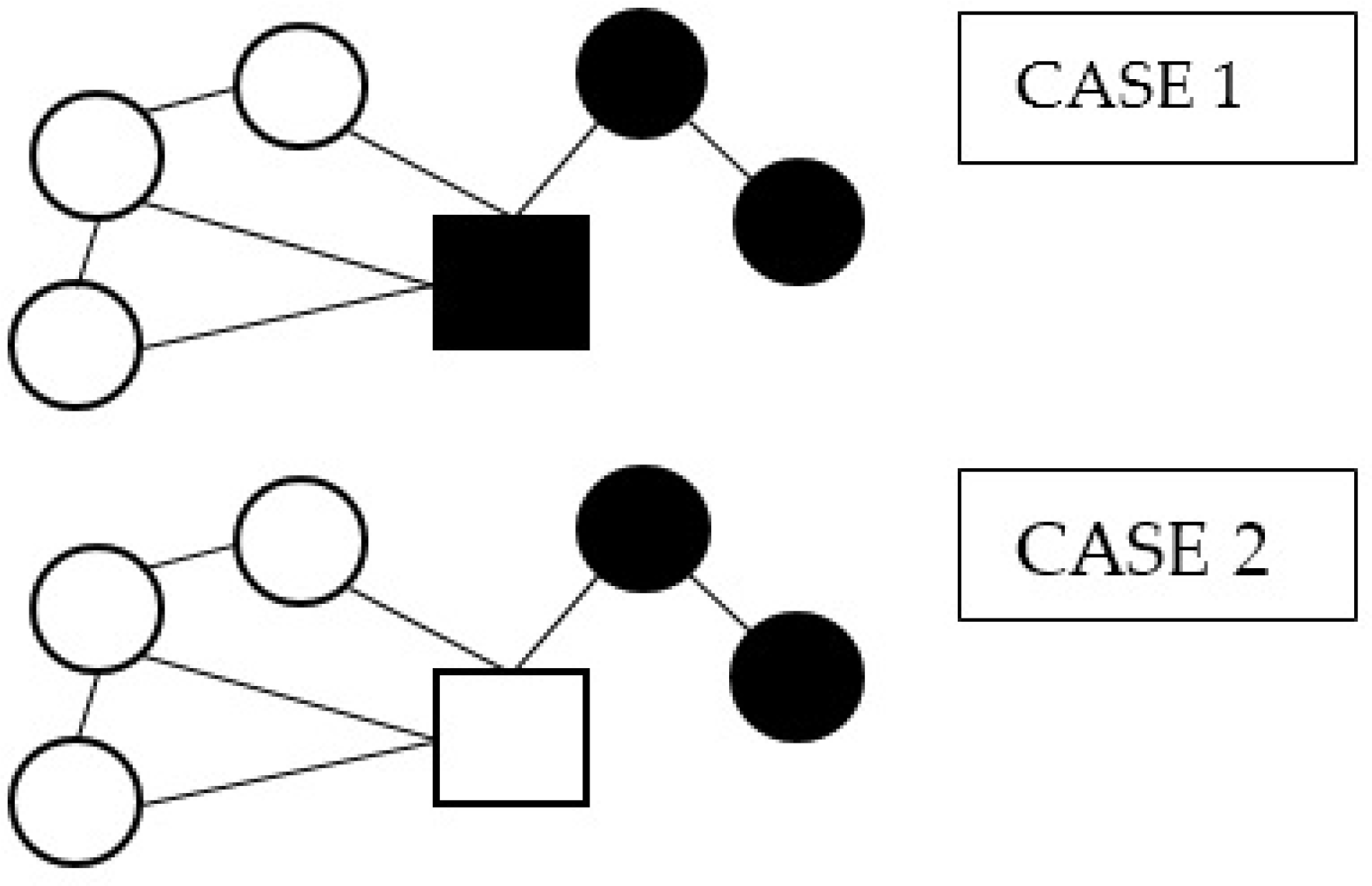
Two partitioning approaches for subsets
Due to the nature of the planning component of the algorithm, the maximum group size is limited. In practice, a maximum size of 20 nodes per planning event was found to be efficient. Groups over 20 were found to increase the computation time and significantly increase the memory requirements.
The harvesting route was determined offline, prior to the harvest occurring. Due to environmental factors, the crop may change between the plan being created and executed. For example, wind or rain might damage or remove certain parts of the crop. To account for changes in the crop in real time, an online implementation should be developed to work in tandem with the offline plan. This would allow the offline plan to evolve with changes in the field as and when they are discovered.
It is assumed that the operator intends to harvest all nodes. A complete harvest may not always be the intention due to factors such as ripeness or health. Currently, there is no provision for including nodes that assist with mobility but are not intended to be harvested. Such a feature would increase the agility of machines such as that in the case study, as well as produce a higher quality yield.
An algorithm, KPSPP, has been developed to generate routes for autonomous harvesting robots. The proposed algorithm has been shown to be effective for the planning of discrete crops in three dimensions, which was not previously available. A case study of an autonomous tree-to-tree felling machine was formed. The study tested the algorithm in 14 different plantation forests with up to 36,000 trees. In the tests, the KPSPP algorithm outperformed all other algorithms in larger sets, with a mean coverage of 84.43% for 3,500 to 36,000 nodes. With a tighter standard deviation (4.16 percentage points) than the next best competitor (18.56), the algorithm proved effective and robust for planning large sets. Performance of the proposed method at lower set sizes (100 to 1,000 nodes), was less competitive where other, existing methods proved equally viable. Increasing performance in smaller sets and refining the subset-formation methodology remain as subjects for future work.