
Abstract
Simple and efficient geometric controllers, like Pure-Pursuit, have been widely used in various types of autonomous vehicles to solve tracking problems. In this paper, we have developed a new pursuit method, named CF-Pursuit, which has been based on Pure-Pursuit but with certain differences. In CF-Pursuit, in order to reduce fitting errors, we used a clothoid C1 curve to replace the circle employed in Pure-Pursuit. This improvement to the fitting method helps the Pursuit method to decrease tracking errors. As regards the selection of look-ahead distance, we employed a fuzzy system to directly consider the path's curvature. There are three input variables in this fuzzy system, 6mcurvature, 9mcurvature and 12mcurvature, calculated from the clothoid fit with the current position and the goal position on the defined path. A Sugeno fuzzy model was adapted to output a reasonable look-ahead distance using the experiences of human drivers as well as our own tests. Compared with some other geometric controllers, CF-Pursuit performs better in robustness, cross track errors and stability. The results from field tests have proven the CF-Pursuit is a practical and efficient geometric method for the path tracking problems of autonomous vehicles.
Introduction
An autonomous vehicle can drive by itself with necessary sensors, such as GPS, IMU, cameras, and Lidar. Normally, the process is that the vehicle first detects the environment and positions itself according to these sensors, and then navigates with global and local planner; finally, the vehicle drives by sending the control commands from the path-tracking controller to the executing mechanisms. With consideration to the process described above, we can see that the path-tracking controller is a bridge that connects the upper software and the lower hardware. As far as the regular definition is concerned, we followed the definition of M. Snider [1]: Path tracking refers to a vehicle executing a globally defined geometric path by applying appropriate steering motions that guide the vehicle along that path. A good path-tracking controller minimizes the lateral distance and heading between the vehicle and the defined path. In this paper we will introduce our latest accomplishments in designing a performance geometric path-tracking controller.
Literature Reviews of Path Tracking
Control Theory Controllers
Pan Zhao [3] proposed a adaptive PID controller to track predefined paths. S-J Huang and G-Y Lin [2] proposed a fuzzy controller to help track the path used to finish reverse direction auto-parking maneuvers. Abbas, Muhammad Awais [4] made the MPC controller run online to track a planned path, which had the capability of avoiding obstacles. While these controllers can promise fine accuracy, PID controllers always suffer from the optimization of parameters and overshot in tracking; the fuzzy controllers need more prior knowledge, and MPC will cost more in computational resources to get a better result. Some literature related other elements to improve the tracking performance. Zhenping Sun [26] used the road information and the state of vehicle to optimize the curvature and then calculated the steering output. Braconnier [27] improved the stability of mobile robots in harsh conditions by deriving the tracking law from the kinematic model. The sideslip angles required by model must be estimated online and also the velocity provided by an adaptive and predictive velocity controller. While more variables could optimize the tracking controllers, it also increased the complexity and decreased robustness of the tracking system. Compared with control theory controllers, geometric controllers are more popular in autonomous vehicles.
Geometric Controllers
Geometric controllers are one of the most popular path tracking methods applied in mobile robotics. These controllers exploit geometric relationships between the vehicle and the path, resulting in control law solutions to the path-tracking problem. The Pure-Pursuit controller is the first geometric controller applied in autonomous vehicles and is also the most widely used. Actually, the earliest Pure-Pursuit controllers were used in regard to the problem of a missile pursuing a target [5]; in the Pure-Pursuit course, the missile's direction of velocity is always pointed to the target position. Pure-Pursuit originated from Wallace et al. [7]; although Wallace did not propose the formal Pure-Pursuit, he used the lateral displacement of the road's centerline from the center of the cameras' forward field of view to compute the steering angle of the front wheel of the vehicle. Based on Wallace's method of analysis, Amidi [6] proposed the ‘Pure-Pursuit’ strategy and discussed its application. Coulter [8] detailed the implementation issue of Pure-Pursuit; since then, Pure-Pursuit has been widely applied in indoor [9] and outdoor robots [10, 11].
In addition to applications, some literature also focuses on the stability of Pure-Pursuit. Anibal Ollero [12] analyzed the relationship between the look-ahead distance and stability. We can conclude from [12] that in order to keep the system stable we must choose a look-ahead distance greater than 1 when tracking a straight path; for a constant curvature path, the look-ahead distance should be greater than 1 and will increase along with the curvature and the delay. Murphy [13] focused on the effects of time delays.
Anibal Ollero [14] also employed fuzzy logic to tune the look-ahead distance. MIT proposed a simplified adaptive method that tuned the look-ahead distance with the velocity. The tuning method's parameters were obtained from a number of different experiences [15, 18],
Unlike the above improvements, which did not change the principle of Pure-Pursuit, Jeff Witąŕs method chased a goal point ahead of the vehicle, but used a different method, vector pursuit [16]. As screw theory can be used to describe the instantaneous motion of a moving rigid body relative to a given coordinate system, it can also be used to represent the motion from the current location to the desired position and the orientation on a given path. Jeff Wit also compared the effect of vector pursuit with Pure-Pursuit and follow-the-carrot. Although the result is that the vector pursuit will be more robust and accurate in tracking different shaped paths, these tests are conducted at very low speeds. According to the method mentioned in [16], the computational process of vector pursuit is more complex than Pure-Pursuit, and more parameters need to be tuned if we want to attain good performance. In addition to the current location, another geometric controller, the Stanley method [17], uses orientation information to compute the steering angle. The Stanley method separately considers the heading error and the distance error between points at the center of the front axle and the nearest path point from the center of the front axle. It then transfers the distance to angle metric with a tangent function. The final steering angle comes from adding the result of the two errors. This method helped Stanford to win the DARPAR champion 2006. Jarrod M. Snider took tests using the Stanley method with some simple maneuvers by Carsim, a type of simulation software. While it can maintain good tracking performance, the tracked path must be a smooth path and its robustness is not as good as Pure-Pursuit [1].
In summary, compared with other geometric controllers, Pure-Pursuit demonstrates better robustness and real-time, which is suitable for autonomous vehicles. However, it also suffers from poor accuracy or possible oscillation when adapting constant look-ahead distances. The MIT method argues that changing the look-ahead distance with the command velocity will improve these problems, but this method does not take into consideration the curvature of the path. In this paper, we also want to develop a pursuit method, based on Pure-Pursuit, but we will differ from prior methods in tuning the look-ahead distance and computing the steering angle. We named our method CF-Pursuit: the Pursuit method with a clothoid fitting and a fuzzy controller to tune the look-ahead distance. As a new geometric controller for autonomous vehicles, we will show CF-Pursuit's superior performance by comparing it with other classical path trackers for vehicles, like the MIT method and the Stanley method.
We have arranged this paper as follows. Section II first reviews the autonomous vehicle model. In Section III we will introduce the method of original Pure-Pursuit, MIT, and Stanley method, and then an analysis will follow regarding the geometric method. Section IV proposes CF-Pursuit and several pieces of literature relevant to the fitting methods. In section V, we will show the experience results to compare CF-Pursuit with the MIT method and the Stanley method. Finally, the paper will include conclusions and references.
Robotic vehicle model
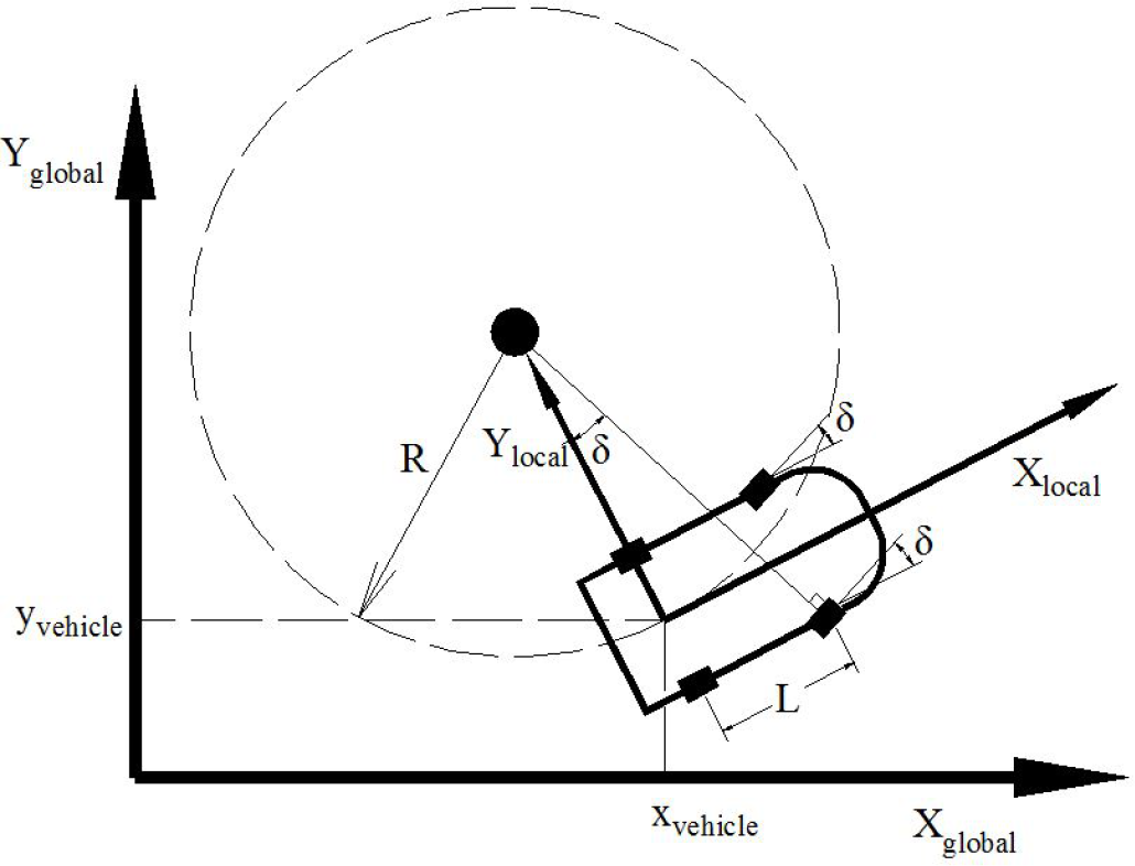
Fig. 1 shows the global coordinate system and the local coordinate system the origin of which is located at the center of the rear wheels. We used X global , Y global to represent the global coordinate, and x local , y local to represent the local coordinate. Ignoring the motion of z axis, we can express the motion state of the vehicle as position and orientation (heading), q = [x,y,θ]. The kinematic model of the robotic vehicle is expressed as:

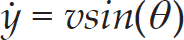

where x,y is the position of the vehicle, θ is the vehicle's heading, as shown in Fig. 1. According to Equations (1), (2), (3), the main task regarding tracking is to calculate the curvature κ, velocity v. The backward motion is not taken into consideration and the dynamic effects such as side slip are ignored for control design purposes. As a result, the Ackerman geometric relationship, equation (4) can be employed to calculate the curvature. And equation (3) can be rewritten as equation (5):


where the Δ is the steering angle of the front wheel, L is the vehicle's wheelbase, R is the tuning radius and κ is the tuning curvature. Differ with the whole vehicle model in Fig. 1, we must simplify the vehicle into a classical bicycle model, shown in Fig. 2 so that the equation (4) can be applied.
Actually, Fig. 1 also shows the principle of Pure-Pursuit. When the vehicle turns with a fixed steering front-wheel angle, the vehicle's path will be a circle with an approximately constant radius. Conversely, when you specify a circular path for the vehicle, you can also calculate a steering angle for the vehicle to track the circle. In the next section, we will provide more detail about Pure-Pursuit.
Global coordinate system (X global , Y global ), local coordinate system (x local , Y local )
A general method for geometric tracking controllers is to pursue a position ahead of the vehicle with a look-ahead distance, and then calculates using geometric methods to connect this position with the current position of the vehicle. For example, Pure-Pursuit uses a circle curve to fit two positions, and Vector Pursuit uses screw theory.
Pure-Pursuit
The principle of Pure-Pursuit is to calculate the instantaneous curvature of the path that the vehicle intends to generate with the current velocity and heading. We use Fig. 2 to show the detail of Pure-Pursuit.

Geometric explanation of Pure-Pursuit
Combining our own experiences and the original description in [8], we can detail the implementing process of Pure-Pursuit as follows:
Find the current location of the vehicle in the global coordinate system (x vehicle , y vehicle );
Find the closest point on the path to the vehicle, (X cv , Y cv ) which is used to locate the vehicle on the path, at which point we can search from it;
Choosing a constant look-ahead distance and then search the goal point (X la , Yla);
Transform the goal point to vehicle coordinates (x la , y la );
Calculate the curvature and then acquire the steering angle from Equation (9);
Update the vehicle's position and recycle.
The Stanley method is a path tracking approach used by Stanford University in the DARPA Grand Challenge. The parameters employed in the Stanley method are shown in Fig. 3. This method firstly finds a nearest point (c x ,c y ) from the front wheels on the defined path, and then calculates the perpendicular error e fa and the heading error θ e :
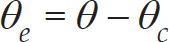
where θ is the vehicle's heading and θ c is the heading of the path at (c x , c y ). the Stanley method is expressed as follows [17]:


Parameters used in the Stanley method
In order to rapidly converge to the defined path, the Stanley method not only considers the heading error, but also transfers the perpendicular error between the vehicle and the path into an angular error in order for the vehicle to quickly intersect with the path.
The MIT method can be seen as a variant of Pure-Pursuit; the definition of variables can be seen in Fig. 4.

Definition of variables. Two shaded rectangles represent the rear tire and the steerable front tire in the bicycle model.
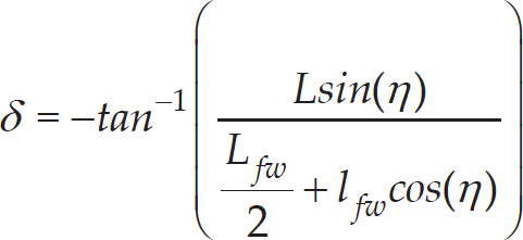
In this method, the original point of local coordinate system is not located at the center of rear wheels; instead it's located at the anchor point. Therefore, the computational method of the steering angle Equation (13) is also different from Pure-Pursuit. According to its analysis, this change will improve stability. Another improvement relates to the look-ahead distance. The look-ahead distance will change with the velocity, the command velocity [15]. The specific tuning mechanism can be obtained using the following expression:

For the geometric controllers applied in vehicle, the geometric relationship between the two positions consists largely of 2-D curves, such circles and polynomials. Therefore, from a geometric point of view, there will be three curves demonstrated from the initial calculation to an actual trajectory of the vehicle. The first is the defined path, the second is the curve representing the relationship between the two positions, and the third is the real path that the vehicle intends to follow. We show this process in Fig. 5. As such, the cross track error Error cte can be expressed as Equation (14):

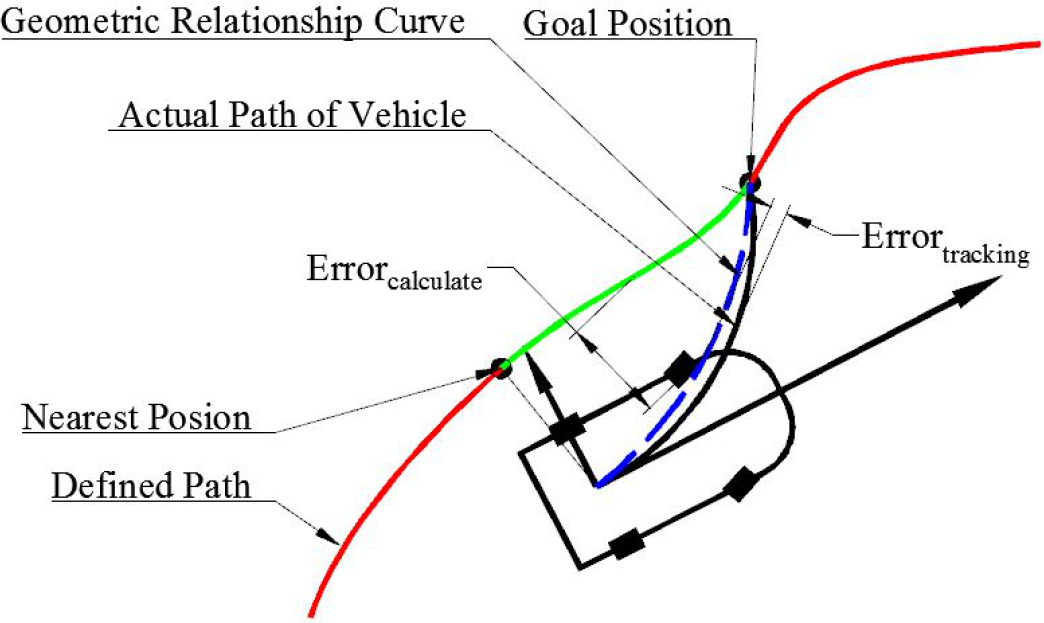
The blue dash line represents the geometric relationship between the starting position to the goal position. The black solid line is the actual path of the vehicle generated when executing the control commands.
Here, we have defined the Error tracking as the errors brought by the procedure when the vehicle executes the control commands. If the autonomous vehicle has finished the adaptation, the Error tracking should be constant. Another Error calculate indicates the errors caused by the truth control value and calculated value through algorithms. As to geometric controllers, the calculated control value depends on the geometric curve. In fact, the geometric curve can be seen as a fitting curve for the part of the defined path, starting at NearestPosition and ending at GoalPosition. Moreover, the Error calculate is affected by the fitting effects; the fewer fitting errors there are, the lower Error calculate is. Amidi [6] already discussed this problem, proposing a quintic polynomial to fit the origin and the goal pose. In every pose, there are four dimensions; in addition to position, the orientation and curvature are also required. The experience's results demonstrate that this method can obtain a better tracking performance, but the computation is too complex, and the computing success rate cannot be guaranteed because of the number of constraints and parameters. However, we can conclude that there are two core directions in optimizing a geometric method; one is to find an optimal GoalPosition using the look-ahead distance, the other is to employ a better fitting method to decrease the fitting errors. The MIT method and some other methods that focus on optimizing the look-ahead distance try their bests to solve the problem of how to select a GoalPosition to generate a circle by Pure-Pursuit. However, this means they ignore another problem: the optimization of the fitting method, which is also important to decrease Error calculate . According to the fitting theory, better fitting effects can be achieved when considering more constrains. Nevertheless, too much constrains may result in difficulties in the calculation. For CF-Pursuit, we tried to improve on the fitting problem based on a newly developed fitting method, the new clothoid fitting. In the matter of selecting GoalPosition, the fuzzy strategy was adopted to tune the look-ahead distance. Different from the other tuning methods [14,15], we were concerned only with the curvature of the path, instead of the velocity.
Some of the literature has attempted to improve tracking effects by using better fitting methods. Vicent Girbĺęs employed the combination of clothoid curve, line and circle to fit the tracked path [19]. In order to handle any possible fitting failures, the original Pure-Pursuit will be used if a failure is detected. The fitting method for CF-Pursuit is similar to the principle of this paper, but we will argue the necessity of fit using a Continuous-Curvature curve. The success rate is hard to promise when considering four dimensions [6]. Even in [19], Pure-Pursuit was used as an alternative method when it was impossible to converge. On the other hand, the drawback addressed by [19] is the uncomfortable feel that comes from abrupt changes to the heading. According to our experiences, while maintaining continuous curvature is helpful for smoothness of control, it will weaken the fault-tolerance of the whole system. For example, when huge blocks hide the GPS, the location accuracy will be poor and the autonomous vehicle will become lost and will deviate from the defined path. Once the system recovers from a worse situation, out of consideration for safety we need the vehicle to return to a normal course as soon as possible. However, this process may take longer if we consider the curvature continuity, given the possibly enormous gap between the fitting curve and the defined path. In actuality, a sudden change in heading can be caused by many factors, and curvature discontinuity in tracking is just one of them. If we can have tracking errors limited to a narrow range and maintain control over speed, there is a low probability for a sudden change of heading even if you employ a controller that does not consider the curvature continuity. [28] expended [19], besides of the DCC path, [28] also generated a speed profile based on “slow in” and “fast-out” policy to improve the original method in [19]. Nevertheless, [28] did not create any innovation in generating DCC path, so the above mentioned problems still existed. In the CF-Pursuit, we employed the clothoid curve to fit, but without a line and circle. Accordingly, we did not want a continuous curvature curve; instead, we considered the two given positions with signed tangent vectors. In terms of fitting effect, this is better than a circle, but worse than a continuous-curvature curve. Nevertheless, we can guarantee a high success rate when we employ the new calculation method [21]. We also did not need an alternative algorithm based on our tests. On the other hand, the results using clothoid will be used in the later fuzzy system to tune the look-ahead distance. In order to better illustrate this, we must first introduce the clothoid curve.
Clothoid Curve
The general parametric form of a clothoid spiral curve is as follows:
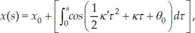

where s is the arc length, (x0, y0) is the starting point and θ0 is the initial angle. Notice that 1/2 κs2 + κs + θ0 is the angle of the curve at arc length s. As far as we all know, the clothoid curve is computed via the Fresnel sine and cosine integrals [20]. The determination of the parameters θ0, κ and κ are calculated by points and angles at the extremities of the curve.


In addition to the above constrains, we all want the whole length of curve L to be minimal, allowing us to solve the parameters, θ0, κ and κ from the following nonlinear system [20]:

In this paper, we followed the method proposed by Enrico Bertolazzi and Marco Frego, which provides a robust and fast computational method [21]. Unlike other calculation methods, this new method does not need to split the problem in mutually exclusive cases as the method in [22], and also does not suffer in case of degenerate Hermite data like straight lines or circles. We used an example to explain the benefit of employing clothoid, but not Hermite or other polynomial fitting methods. In this example, we chose two points on a circle with a 10 (m) radius, centered at (0,0), and then we separately employed clothoid and Hermite to fit. We found nearly the same overlap ratio and shape-preserve in the left of Fig. 6. According to the requirement of Equations (9), (10) we needed to calculate the curvature at the present position, which was the starting curvature of the fitting curve. To this example, we found the curvature's curve in the right of Fig. 6. Compared with clothoid, Hermite does not get a constant curvature, and the curvature changes abruptly, but clothoid can almost obtain a constant curvature like a circle.

A comparison between common Hermite and the clothoid fitting
Methods
The selection of GoalPosition is also important to geometric controllers and depends on the look-ahead distance. Longer look-ahead distance will have the vehicle gradually converge to the path with less oscillation, and the shorter distance will converge fast but possibly with more oscillation. A. Ollero used a fuzzy supervisory to tune four parameters in his system [14], including a look-ahead distance. In his fuzzy system, four variables were considered to be the inputs: the distance from the vehicle to the nearest point in the path to be tracked, the actual velocity, the curvature at the goal point, and the difference between the heading of the vehicle and the heading of the nearest point in the path. In later practice, the MIT method proposed that it was good enough to consider only the velocity. While the MIT method does a good job in its autonomous vehicle, this method depends on the velocity control also does not consider the curvature of the path.
When we tune the look-ahead distance, the most important element is the curvature of the path [8]. Essentially, the look-ahead distance changing with velocity merely reflects its dependence on the curvature of the path. For example, as a simple velocity strategy, decelerating speed indicates the forward path may be curvy, while an acceleration means a straight path. Nevertheless, the curvature of the path cannot be totally represented by the velocity, which can be affected by other traffic elements. As a result, we want to develop a tuning method that can tune the look-ahead distance through the curvature of the path ahead. In order to calculate the curvature of the path ahead, the clothoid method must be employed again for this process. Instead of fitting the whole defined path off-road, we fit it in real-time. We used the maximum curvature of the fitting curve to decide the curving degree of the fitted path. However, we must consider the credibility of employing a characteristic of the fitting curve to represent the fitted curve; great fitting errors may make it distorted. As such, we took two measures to handle this problem. The first was to limit the length of the fitted curve and test to find an optimal maximum length in order to reduce the chance of great fitting errors. The second was that we chose multi-goal points in the defined path to fit, and then used a fuzzy controller to integrate the curvatures obtained from the calculations of the clothoid fitting to decide the specific look-ahead distance.
Fuzzy controller
By far, there is no mature theory or model to define the relationship between the curvature of the defined path and the look-ahead distance. And also there is not a clear definition regarding the degree of curve of the path. What we have now are just the drivers' experiences and some of our own testing experiences. While lots of the accurate control methods can be employed, only the fuzzy method does not require a complete mathematical model of the controlled system. Moreover, fuzzy logic can reason approximately, which is particularly well suited to handle imprecision and uncertainties. In particular, Sugeno and Nishida demonstrated that fuzzy control was capable of handling nonlinear control problems using oral instructions [23]. Lastly, the computational efficiency of fuzzy controllers allows real-time operation which is a critical requirement for the autonomous vehicle.
From a formal point of view, a fuzzy controller consists of a rule base containing the experts' procedural knowledge and a variable base containing the different linguistic values. As regards the experts' procedural knowledge, we obtained two kinds of knowledge: human drivers' experiences and experiences of our tests, which are all listed as follows.
Human Drivers' Experiences:
We will focus on a short distance from the host vehicle and tune the steering wheel finely to avoid the vehicle going off the road when the visible road ahead is curvy.
We will look ahead as far as we can from the host vehicle when we can see the road ahead is straight.
Our Tests' Experiences:
We need to shorten the look-ahead distance when we turn or if the defined path is very curvy.
We need to extend the look-ahead distance when the defined path is not too curvy.
A minimum look-ahead distance 6 meters and maximum 12 meters were tested and found to be proper when controlling the speed of vehicle to be under 30 km/h.
We can approximately define the path curves when the curvature is bigger than 0.1;
We can trust the curvature value in 12 meters ahead if the calculated curvature is very small;
Fuzzy rule base: Neither the human drivers' nor our tests' experiences can be used directly to form the rule base; they require normalization. In addition, they only frame the control process, but not any detail of how to maintain control. Consequently, we need to enrich them. The rule base to tune the look-ahead distance is:
IF 12mcurvature is
F 12mcurvature is
F 12mcurvature is
F 9mcurvature is
F 9mcurvature is
F 9mcurvature is
F 9mcurvature is
F 9mcurvature is
F 9mcurvature is
IF 6mcurvature is
IF 6mcurvature is
IF 6mcurvature is
IF 6mcurvature is
Fuzzy variables: the words in italics are the fuzzy input and output variables, and the words in bold are their associated linguistic values. We chose three GoalPositions, separately from the host vehicle: 6 meters, 9meters and 12 meters in advance. Based on our experiences and referring to [15], 12 meters is a proper upper bound of look-ahead distance with the velocity lower than 40km/h. The curvature at 9 meters makes the change of curvature with respected to length smooth. These three variables have four associated linguistic values(small, middle, large and larger), each with their respective membership functions. The shape of the membership function depends on how much we want them to affect the control. Lastly, we also define a fuzzy output variable, the lookaheaddist, whose linguistic labels are (short, middle, long and longer).
Fuzzy rules: When the curvature in 12 meters is small, we trust that the fitted path within distance of 12 meters is not curvy. This is what rules 1 and 2 represent. When 12mcurvature becomes large or larger, we trust that the tracked segmental path is curvy, and the 12mcurvature cannot represent the fitted path because of possible greater fitting errors. The 9mcurvature and the 6mcurvature will take effect together or alone. This process can be represented by rules 3 to 13.
From a functional point of view, the fuzzy reasoning process can be divided into three stages, shown in Fig. 7, fuzzification, inference engine, and defuzzification.

Structure of a fuzzy system
Fuzzification: In this step, current crisp input values are transformed into linguistic or fuzzy values that can be interpreted by the fuzzy compiler. This transformation computes a degree of truth for each of the input fuzzy variable values, depending on the shape of their associated membership functions. We transformed three curvatures into fuzzy values.
Inference engine: The inference engine propagates the matching of the conditions to the conclusions, generating the contribution of each rule to the control action. In our case, Mamdani ¡−s [24] inference method (min-min-max) was used to solve the fuzzy implication.
Defuzzification: Defuzzification is the transformation of the output fuzzy values that were generated by applying the inference method into crisp values that could be used to output control intentions. In this instance, we use the center of area (CoA) method, i.e.,

where ω i represents the membership degree resulting from the inference of the ith rule, and B i is the membership function for the different values of the output variable of the ith rule.
We have defined the output fuzzy variable membership function shapes using Sugeno ¡−s singletons [25], which uses monotonic functions. A modified CoA Equation was applied, i.e.,

Therefore, the y CoA ′ is just the look-ahead distance.
Fig. 8 shows the definition of functions for three input variables, each with the four same linguistic labels (small, middle, large, and larger). They depend on the curvatures calculated from three different GoalPositions. According to our previous tests, 0.1 is a proper break point when using curvatures to differentiate the curvy degree of the defined path. As a result, in Fig. 8 when the curvature is greater than 0.09, the membership to

Membership function of three input variables, Trapezoid is employed
We also used Matlab to show the rule base in Fig. 9. As you can see from the image, the input variable 6mcurvature is referred less frequently in the rule base compared to other two variables. Indeed, the minimum look-ahead distance will be employed less during urban driving unless the vehicle needs to turn around or maneuver sharply.
Platform
We ran a field test to demonstrate that CF-Pursuit will take effect and perform better than the other controllers. The field test was conducted on a free road, which was newly built. The platform we controlled was the autonomous vehicle belonging to Wuhan University, Tuzhi, which had won the third price in “The 2010 Future Challenge: Intelligent Vehicles and Beyond” competition. At the time of the field test, Tuzhi had been improved with advanced Lidars, Cameras and a location system. On the other hand, a variety of new algorithms regarding sensing and control were also applied. The hardware and software architectures of Tuzhi are shown in Fig. 10.

The fuzzy controller we used Matlab to simulate
Defined Path
In order to make the test less affected, we did not employ too many sensors to support our experience. We used only the GPS and IMU to collect location data to compose a defined path Pathτ, and then automatically drove the vehicle to follow the Pathτ. This Pathτ was generated when a human driver drove a car along a road, and that path was then saved in the computer. Our GPS and IMU system is fine and stable in accuracy, about ±0.02 meters in open area. We chose a location with fewer people, trees and high buildings, thus mitigating the likelihood of poor GPS accuracy. We also took a screenshot from Google-earth, shown in Fig. 11.
In the Pathτ, we included five urban driving maneuvers: go-straight, lane-change, turn-left, turn-right, and turn-around. In order to get better results in path tracking, another important element, the velocity must also be considered. In the MIT method and the Stanley method, the velocities were all considered in their algorithms. However, the, CF-Pursuit does not consider velocity, which is a challenge we want to face. In this test, we did not design a fine velocity controller; we set the go-straight and lane-change velocity as 20–30 km/h, turn-left and turn-right as 15–20 km/h, and turn-around as 5–10 km/h. To the speed controller, we just used a simply P-Controller to control it. The purpose of this paper was to design a steering controller, not a speed controller. Consequently, the task of a speed controller was to make sure three methods were tested with the same velocity profile over the whole path. Nevertheless, we needed to manually engage the vehicle's brakes when the vehicle encountered danger or if we sensed a dangerous situation may occur, like collisions with curbs.
Compared methods
The geometric controllers updated slowly in recent year, especially the controllers applied in autonomous vehicles. As for compared methods, we choose the MIT and Stanley method, which were popular among the pursuit methods applied in the autonomous vehicles. Another reason to choose them was that both of them were tested in the DARPA and helped the corresponding vehicle obtain a good place. In term of controller's properties, these two methods are both coupled with velocity, and then affected by the control of the velocity, the CF-Pursuit will decouple the velocity in the steering control. The challenge here is that we want to behave better without consideration to velocity, like with the MIT and Stanley methods. With regard to certain unknown and tunable parameters in these two methods, we tried our best to make sure the parameters were optimal so that the uncertainties could be decreased and the algorithm could perform to its true potential.

Left: Tuzhi is taking part in Challenge of Intelligent Vehicle in China 2014. Right: Simple software structure of Tuzhi.

Screenshot from Google-Earth: the purple, while and green paths are separately associated with velocity 25–30 km/h, 15–20 km/h, and 5–10 km/h
Unlike high velocity applications, we focused on the curving and middle velocity situation. In actuality, high velocity applications imply that the path is flat. On the other hand, we need to consider the dynamic effects such as side slip when we drive at high speeds, which is difficult for the geometric controllers to apply currently. This paper tries to solve for urban applications, requiring the autonomous vehicle to perform common urban maneuvers like turning left or right, turning around and changing lanes. We have shown the whole velocity profile of applying these three methods in Fig. 12. In order to avoid possible collision with curbs we have to brake the vehicle to slow it down within the ellipses areas. For the MIT method in (a), this only happened when we nearly finished turning left. The minimum velocity we must control manually is under 5 km/s; however, the steering angle is always tuned automatically. As to the Stanley method, we applied the brakes more to tune the velocity and in addition to the turn, we had to control the speed manually until completing turn-around. Even worse, there were two positions in (b) that required us to stop the vehicle and steer manually. By comparison, the CF-Pursuit in (c) not only maintained a higher speed but also completed the whole test without any manual interruptions.

Actual paths with corresponding velocities when applying the MIT method (a), the Stanley method (b), and the CF-Pursuit (c) separately
Another performance we want to compare is the stability of algorithms. Instead of complex measures for some standard parameters, we used the steering angle to reflect stability. The results are shown in Fig. 13. When controlling acceleration and deceleration gradually or maintain a constant speed, the MIT method is the best for stability, and the Stanley method is the worst of the three methods. However, focusing on the green ellipses in Fig. 13(a), an abrupt change in the steering angle has been triggered; the result is a sudden change in the vehicle's heading. This kind of driving behavior is dangerous and uncomfortable for the passengers within the vehicle even if it only happens once. A reasonable interpretation of this is the MIT method only tunes the look-ahead distance with the velocity, but not with the curvature changes in the path. In this example, we could associate a greater than expected velocity when it turns left; as a result, the cross track errors would increase when the path begins to curve (Fig. 14 (a), (d)). Once we manually slow the vehicle to an expected velocity, which would indicate a curvy path ahead, the look-ahead distance is consequently shortened, and then the algorithm would try to compensate for the errors as soon as possible. The final result is a sudden change in the steering angle. Looking at the Stanley method (Fig. 13 (b)), oscillation is a typical characteristic. Unlike the MIT method, the velocity directly acts on the algorithm (Equation (12)). When experiencing this method, we need to consider two problems. The first is that we must handle the issue of zero velocity by letting velocity be equal to one when the velocity is zero. The second is the relationship between parameter k in Equation (12) and the velocity. A constant value was chosen based on our tests. In actuality, we can also treat the Stanley method as a kind of pursuit method, as it pursues the (c x , c y ) in Fig. 5. Oscillation may be related to the choice of k, however, from the view of the Pursuit principle, choosing a nearly constant and short look-ahead distance will also result in oscillation. Another possible reason is that the algorithm is sensitive to the e fa (Equation (12)), which will always exists no matter whether dealing with a straight or curved path. Applying this method, the actuator will control the steering wheel only if the e fa is nonzero. We also can see in Fig. 14(b) that the oscillations' sensitivity will change with velocity. The two paths within the red ellipse in Fig. 14(b) are both straight roads, but one is more stable than the other. Referring to Fig. 13(b), differing velocity profiles is the main reason for this. Also, the Stanley method keeps the greatest cross track errors obtained from Fig. 14(b)(e). By contrast, While the CF-pursuit method does not perform as well as the MIT method with regards to stability in some of situations, there is no sudden change like in the MIT method; also, when we refer to Fig. 14(c)(f), we can find that small fluctuations are helpful in controlling the cross track errors. Actually, we did not feel uncomfortable at all in the vehicle.
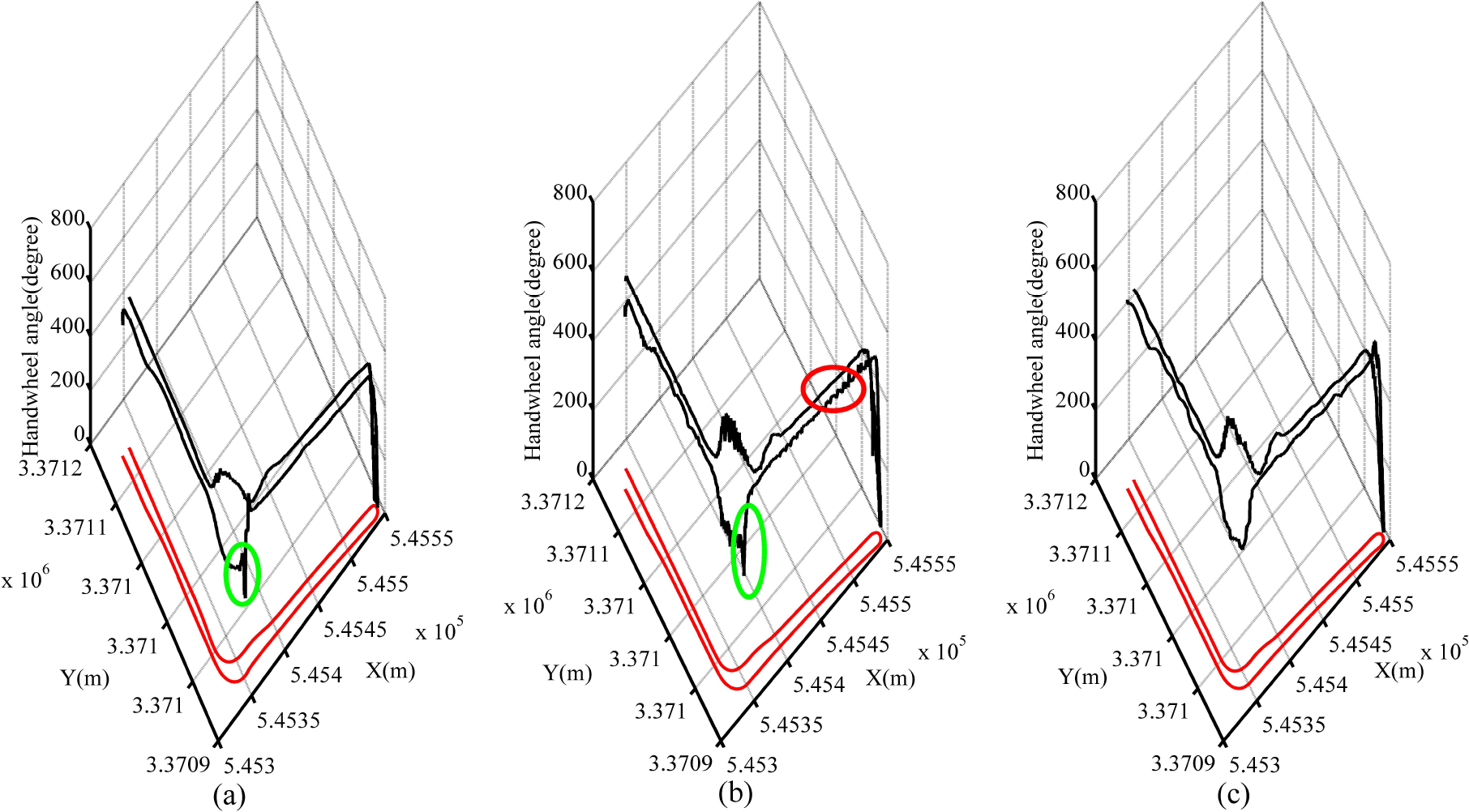
Actual paths with corresponding steering angles when applying the MIT method (a), the Stanley method (b), and the CF-Pursuit (c) separately

Actual paths with corresponding steering angles when applying the MIT method (a), the Stanley method (b), and the CF-Pursuit (c) separately
The CF-Pursuit method makes use of the clothoid fitting method to decrease the fitting errors and designs a fuzzy controller to tune the look-ahead distance. Driving experiences demonstrate that it is a better tracking algorithm in the velocity's robustness, stability and cross track errors. Nevertheless, we also found that it was not as stable as the algorithm that considers velocity while tuning the look-ahead distance when driving on straight path and controlling the velocity properly. As such, integrating the curvature of the path and the velocity together may be an interesting direction for any further research. On the other hand, limiting the length of a fitted path to weaken the effects of the fitting errors may make it impossible to accommodate more complex situations. However, longer distances mean possible greater fitting errors, which also have to be considered in the future.
Footnotes
6.
We would like to acknowledge Jian Zhou, Ling Zheng, Liming Fu, Zhi Lu, Xiaomin Guo, Wei Yang Yuan Guo and Cheng Chen for their contributions in developing the autonomous vehicle. The work described in this paper is supported in part by National High Technology Research and Development Program of China (2012AA101701).