
Abstract
This article presents an effective solution for the localization of a vehicle in dense urban areas where GNSS-based methods fail because of poor satellite visibility. It advocates the use of a visual-based method processing georeferenced landmarks obtained after a learning path and stored in a new layer of the geographical information system (GIS) used for navigation. Real-time localization gives, with few failures, accurate results in the areas covered by the GIS. The integrity of the localization is obtained by running another algorithm in parallel, processing odometric data combined with the geometric model of the drivable area and, when available, GNSS data in tight coupling. An ellipsoidal confidence domain is updated by using both extended Kalman filtering (EKF) and set-membership estimation. Although less accurate, this estimation is reliable and, when the visual method fails, the availability of a confidence domain enables us to speed up the restart of the visual method while navigating cautiously. A large-scale experiment (>4 km) was conducted in the centre of Paris. We compare the absolute localization results with the ground truth obtained by combining RTK-GPS and a high-end inertial measurement unit (IMU).
Introduction
This article addresses the question of the integrity of the accurate localization of a vehicle in dense urban areas. This topic has many applications, such as ADASs (advanced driver assistance systems), autonomous driving and augmented reality. In recent years, the ego-localization of a vehicle has been based on GPS coupled with odometry or inertial sensors, which has proven to be an efficient solution except in places where the visibility of the sky - and consequently of the satellites - is problematic, for instance in urban canyons in city centres. This is why attention has been paid to other sensing modalities. During the last 10 years, several works have shown that vision can improve the accuracy of urban localization especially in city centres.
The proposed method is based on the parallel execution of two processes. The first one is essentially a map-aided odometric algorithm using when available, satellite data in tight coupling. Due to the simplicity of the odometry together with the generalized use of the GIS, the reliability of the results is almost 100%, but even though all of the available data at each instant and in any place are used, the accuracy is not sufficient for navigation at the level of the lane. The second one is vision-based and makes use of georeferenced visual landmarks contained in a new dedicated layer of the GIS. This technique is accurate but may fail due to some defects or in some areas not covered by the dedicated layer of the GIS. Both methods are iterative and share a common ellipsoidal confidence domain in the 6D configuration space (position + orientation). The size of the domain quantifies the accuracy of the localization estimate.
The principles and the properties of each method will be explicated, their cooperation further exposed, and the whole method will be illustrated by the results of a full-size experiment. With this work, we bring two contributions:
First we present a system which combines information from vision, GPS, odometry and an existing map to localize a vehicle. This localization is accurate most of the time thanks to the vision and, in case of failure of the vision part, it guaranties the integrity of the localization with reduced accuracy. Moreover, when the prerequisites of visual localization are validated again, the continuously updated localization domain enables us to restrict the set of visual landmarks to be considered and thus speeds up the restart of the accurate visual localization.
The second contribution is experimental. We have realized an experiment based on a trajectory passing through narrow streets in the centre of Paris, France. In this context, many papers on visual localization give relative localization results - here, we give absolute localization results and compare them to the ground truth given by combining RTK-GPS and the high-end IMU used for this experiment. We discuss implementation issues and the large amount of processed data which lead us to consider exceptional behaviours of the visual algorithm that emphasize the necessity of its collaboration with another method to achieve the integrity of the localization.
Related Work
Global navigation satellite systems (GNSSs) such as the American GPS, the Russian GLONASS and the European GALILEO, give anyone with an ad-hoc receiver the possibility of being localized in an earth-fixed reference frame. Despite continuous research in enhancing the accuracy and integrity of the localization, when the reception of the pseudo-ranges and Doppler signals broadcast by the satellites are degraded, the accuracy is insufficient to localize the vehicle at the lane-scale. In [1], even though using sophisticated non-linear identification methods together with particle filters in the place of least-squares or Kalman filtering, the experimented accuracy is above 4 m with three visible satellites and 5 m with less than three. The “urban trench” model has been considered since it has been shown that the positioning error is distorted across the street direction [2], but the results of large-scale experiments reported in [3] show that, despite a noticeable gain in accuracy, the localization at the lane level is not achieved.
To overcome the difficulties with GPS reception in urban areas, the research in vision-based localization methods has been very active in the past 10 years. Above all, it is now a matter of common sense to define the displacement tasks with respect to some real elements of the environment, typically a side walk limit or a zebra crossing. Vision referenced control, for the sake of decreasing the cost of artificial vision, is an increasingly widespread technique. More generally, one should note that the accuracy of a visual localization algorithm is improved if it uses visual landmarks close to the camera. In fact, navigation accuracy is needed in places where there are obstacles or road limits near the vehicle. It is precisely in these places that the environment offers a lot of visual features. Note that the problem is the opposite for GPS-based solutions. In urban environments, especially in an urban canyon, the accuracy of the GPS decreases when the one of vision-based methods is enhanced, which makes these two approaches complementary.
A natural idea consists of using a 3D model of the environment stored in a GIS and to match visual features extracted from the GIS for the current image to compute the pose of the vehicle. For instance, Cappelle [4, 5] proposes using a 3D map of a Stanislas square in Nancy (France), where some recognizable elements such SIFT, SURF and Harris points are compared so as to be matched to the same features computed from a virtual image computed from a 3D model managed by a GIS. With those features being referenced in WGS84 coordinates, the vehicle localization deduced from the comparison of the matched points is also defined in WGS84 coordinates. However, the 3D model needs to be accurate and realistic enough to allow for a reliable matching of visual features. Such models are not widely available. Therefore, it is preferable to build a visual landmark database associated with a set of streets by driving a pioneer vehicle through the area in an initial learning phase. This database can be built using visual SLAM (simultaneous localization and mapping) or SFM (structure from motion).
Vision only SLAM has been developed and even made possible for real-time situations in small environments [6]. However, SLAM's complexity is too high for city-sized environments. For vehicle localization, visual odometry is preferred [7] but the drawback of this method is the drift of the localization. Several approaches have been proposed to reduce or completely suppress this drift. Scaramuzza et al. [8] use the non-holonomic constraint of the vehicle to reduce drift. Alternatively, an IMU can also be used to compute the scale of monocular SLAM and reduce drift [9].
In order to obtain a georeferenced localization, it is necessary to integrate additional data in the visual SLAM process. Lothe et al. [10] use a coarse 3D city model to register the visual reconstruction and suppress drift. The 3D model can be replaced by an aerial view [11]. The problem which must be addressed when constructing large-scale visual reconstructions of cities with the integration of either low-cost GPS measurements or GIS databases is the possible lack of accuracy or error of these data. Some authors have proposed methods to integrate this information in a bundle adjustment framework. For example, Lhuillier [12] includes GPS measurements as constraints in the minimization process. Stretcha et al. [13] use a skeleton graph model to reduce the complexity of the optimization process in large-scale reconstructions based on images, low-cost GPS and GIS databases. It is also possible to record high precision GPS data along with images in an initial mapping step. Lategahn et al. [14] use this method and they combine visual odometry and GPS data in an optimization process to produce a reference trajectory and a point cloud of 3D visual landmarks. We do nearly the same in the vision part of our algorithm, but we register the GPS and SFM trajectories differently to further reduce the re-projection error.
The approach that is proposed here uses two concurrent localization processes that continuously update an ellipsoidal confidence domain. The shape of this domain is compatible with statements of accuracy in both Bayesian [15, 16] and set-membership [17, 18, 19] estimation. Bayesian estimation is a classical, well-mastered technique and, in the case of visual-based estimation, the large number of processed data justifies that the visual-based estimation may be considered as a realization of a Gaussian process (with ellipsoidal confidence domains). On the other hand, set-membership estimation is the correct framework to deal with geographic databases in which the geometric statements are verified and guaranteed. Ellipsoidal algorithms make it possible to update ellipsoidal confidence domains in this context.
The structure of the paper is as follows. Variables, notations and the evolution model of the vehicle are introduced in the second section, while the third section presents the experimental context that is of primary importance for this paper. Section 4 then details the visual localization method in three steps: 1) visual database construction, 2) real-time localization, and 3) good results and a few problems to be dealt with. Section 5 details the map-aided with tight coupling GPS/odometry (MATCGO) method, and finally Section 6 explicates how the collaboration of the two methods brings integrity to the global localization process.
Variables, Notations and the Motion Model
The considered tasks are urban travels that are planned in a map and further supervised during their execution by using the elements of the map.
Elements of the GIS
In the present work, a 3D city model of the environment is available in a GIS managed by SIVNav SDK from BeNomad [20]. This software development kit has been designed for applications with augmented reality, 3D map rendering and vision for robotics. It includes tools for both database management and the accurate geometrical description of buildings, roads (actually, streets) and side walks.
Geographical data are provided by the French National Geographical Institute (IGN), in the national French plane projection (Lambert 93) plus the mean sea level (MST) altitude (also called the GIS reference frame). Their accuracy is: 5 cm horizontally and 25 cm vertically in Paris [21, 22]. The components that are added into the GIS for the present study are: i) a layer containing the visual landmarks that are collected in an initial learning step detailed in Section 4.1, and ii) a set of rectangular patches that define the drivable areas of the streets. All the previous and new components of the GIS are defined in the same reference frame.
Vehicle Configuration
In the sequel, the world reference frame is the GIS reference plane in Lambert 93 coordinates, which is assumed to be orthonormal and direct with (east/north/up) aligned axes. Let us denote

where (x,y,z) are the 3D coordinates of the characteristic point M and the orientation angles are Ψ (heading), θ (slope) and φ (bank).
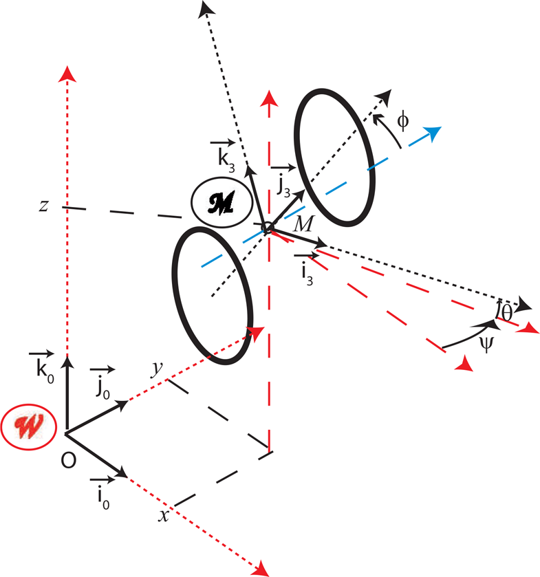
3D vehicle configuration for a fixed rear-axle model, with the world and mobile reference frames, respectively, W and M
In other words, the configuration may be considered as the isometric transformation [0R
m
0T
m
] from M to W, where [0T
m
] is the
Odometric data are now present in any vehicle, whether electric robots or common cars. Using these available data to predict the new configuration after an angular variation of the wheels is a classical way to hybridize a localization in a prediction/update framework. With this aim in mind, we propose to use a simple 3D kinematical model (2) where v (respectively ω) is the longitudinal (respectively yaw) speed.
This model introduced in [23] and developed in [24] is induced from the assumption that the wheels roll without slipping on a tilted planar surface whose inclination is assumed to evolve slower than the other variables. In particular, the slope and bank angles have slower variations than that of the yaw angle. Note that such a model is coherent with the 3D map composed of planar patches that is further used:

A discrete time version for a real-time implementation (3) may be deduced from (2) by the Euler formula:

In this expression, ds k (respectively dΨ k ) is the elementary travelled distance (respectively yaw rotation) between the successive time samples t k and tk+1. Both come from odometric measurements.
Location and Geographic Database
The data comes from the CityVIP [25] validation campaign data. Indeed, in order to finalize the project with a final demonstration, in September 2011 in Paris, a recorded experiment was carried out. Two datasets are available, each one composed by at least two laps (about one kilometre per lap). The first lap is used to build the visual landmark database; the second and further laps are used for evaluation purposes. The urban environment in the vicinity of the 12 th district city hall is very dense, with some narrow streets bordered by high Haussmann-style buildings.
The Vehicle
Both the recorded experiment and the final demonstration of the CityVIP project were performed with the IFSTTAR/MACS vehicle (Figure 2). It was equipped with:
A controller area network (CAN) bus connection (for the odometry);
A low-cost automotive GPS receiver TEA-6T from U-blox (for raw data and NMEA GGA1, GPS fix data and GSV satellites in view, sequences at 4 Hz) and its patch antenna;
The specifically dedicated reference trajectory measurement (RTM) equipment, LANDINS of the IXSEA society, from which the reference trajectory of the present experiment is issued. Its accuracy is about 10 centimetres;
A Marlin video camera with a wide-angle lens.

The experimental vehicle of IFSTTAR/MACS
The data were logged in real-time using a multi-thread software architecture and processed off-line in “replay” mode. The system used to perform these tests was a dual core processor @ 2.53 GHz, 4 GB of RAM and just an integrated graphics controller.
This section presents a technique based upon artificial vision for 3D localization that relies upon a large set of visual landmarks constituting a new layer of the GIS. We propose to first explicit how the visual landmarks database is built.
Building the Georeferenced Visual Landmark Database
With respect to previous works [26] where vision-based localization has been introduced, the originality of the present work relies on the fact that the coordinates of the landmarks are defined in the reference frame of the GIS and not in a reference frame specifically devoted to visual localization. The database is built in an initial learning phase during which video frames are recorded with the onboard camera while the trajectory is recorded with a high accuracy IMU associated with a differential GPS (DGPS) sensor. This initial dataset is composed of a list of (t i ,I i ,IMU i ) for 1 ≤i≤N, where t i is a time stamp, I i is a video frame and IMU i is the pose of the camera according to the DGPS and the IMU. Our goal is to compute C i = [R i T i ] the pose of the camera at frame I i as well as a set of 3D landmarks extracted from the video frames. We cannot assume that C i =IMU i because it is very difficult to estimate the camera orientation with reference to the IMU frame.
Some authors have proposed merging GPS information with the structure from the motion algorithms. For example, Lhuillier [12] proposed a modified bundle adjustment integrating constraints in the optimization process to include positions from a low-cost GPS. It is also possible to directly integrate pseudo-ranges instead of positions in the bundle adjustment as demonstrated by Ellum [27]. In the present paper, more simple techniques are used because an accurate reference path is available. However, this knowledge is not sufficient in itself and some refinements are needed to give more flexibility to the visual reconstruction. In a different context, a similar idea was used as in [28] to improve the quality of the 3D reconstructions from the images.
The solution we used is a global bundle adjustment initialized by the poses recorded in the reference path. More precisely, key frames are first selected in the initial video sequence so that there remains only one key frame for every travelled metre: this reduces the amount of memory and computation time needed and, more importantly, this improves the accuracy of the triangulation. For every key frame, the algorithm is initialized by C i = IMU i . In each key frame, interest points are first detected and then matched through consecutive frames with the Harris corner detector [29] and a zero normalized cross correlation score. Points which are matched on at least two frames are triangulated using the initial poses of the camera. If a point is visible on two frames, a closed-form solution exists. If it is visible on more than two frames, an iterative refinement of the point position is done after an initial triangulation.
This first step gives an initial estimate of both the poses of the camera and the 3D landmarks. These data are further optimized by using a bundle adjustment algorithm [30]. This is done by using the Levenberg-Marquardt algorithm to minimize the re-projection error of every point in every key image according to the cost function F of Equation 4:

The variables which can be adjusted in the minimization are the pose of each camera C i (associated with the projection function π i ) and the 3D position of each visual landmark P j . L i is the set of points visible in the image I i and p i,j is the 2D position of the point P j in image I i . In fact, most of the time, the minimization algorithm does not converge if done directly in this way because the initial error for the orientation of the cameras is too large. The trick consists of first adjusting the orientation of the cameras and the 3D position of the landmarks using the same cost function (considering that the camera position is exact). This first step of the minimization process reduces the mean re-projection error to below one pixel. It is possible to stop the minimization at this step, but in this case the accuracy of the 3D reconstruction (and therefore the localization process) is slightly reduced as illustrated in Figure 3 and 4. It is interesting to further reduce the re-projection error with a full bundle adjustment where the positions of the cameras are allowed to vary. The landmark database we used in this experiment has 856 cameras and 156, 008 points were tracked in the images (an aerial view is shown in Figure 17). If we stop at the first step (left of Figure 3), 123, 476 3D points were correctly triangulated and the mean re-projection error was 0.873 pixels. If we carry out a full bundle adjustment, we get 139, 723 correct 3D points, and the mean re-projection error is reduced to 0.700 pixels. However, introducing this additional degree of freedom implies that the positions given by the vision algorithm are no longer in the same coordinate system as the GIS database.
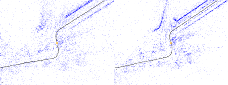
Visual landmark map (top view, vehicle poses in black, visual landmarks in blue). Left side: after partial bundle adjustment (only the angles are optimized), right side: full bundle adjustment (six degrees of freedom for each pose). On the right, building façades are more clearly defined, indicating a more accurate 3D reconstruction.
To overcome this problem, we propose to compute a local transformation from the coordinates defined in the visual reconstruction into the georeferenced ones. This transformation is defined locally in the Frenet-Serret frame associated with the reference trajectory (Figure 5). Given the current position P
vis
of the vehicle in the coordinate system of the vision map, let P0
vis
denote the closest point on the reference trajectory associated with a camera pose, T
vis
being the tangent vector corresponding to the reference trajectory and

View of the area shown in Figure 3

Frenet-Serret frame associated with the reference trajectory
The real-time localization algorithm is designed to compute the pose of the camera from a single image. An initial estimation of the pose of the vehicle is provided by the propagation of the previous estimate obtained either from previous visual data or from map/satellite-based localization, further detailed in Section 5. In this last case, the accuracy of the estimation is about a few metres but it is useful to select a set of candidate key frames on the reference trajectory which are close to the current position of the vehicle. Matching interest points between these key frames and the current image yields associations between 2D points and 3D points in the landmark database (Figure 6). The pose is then computed in a RANSAC scheme to eliminate outliers and is improved with an iterative minimization of the re-projection error [31]. Afterwards, the kinematic motion model (Section 2.3) is used to predict the pose of the vehicle for each new video frame. The process to update the pose of the vehicle is the same:
Select the closest key frame to know which landmarks can be observed;
Match the interest points detected in the current frame to the interest points of the closest key frame;
Retrieve 3D coordinates of the points matched in the key frame from the visual landmark database;
Compute the pose of the camera and the associated covariance matrix.

Interest points matched between the current image (left) and the closest key frame (right). The yellow points are inliers and the red ones are outliers.
When enough interest points are matched between the current image and the closest key frame, the localization is very similar to the reference trajectory as can be seen in Figure 8.
The accuracy of the result is below one metre, as shown in the cumulative distribution function of the absolute error in 3D (Figure 7) computed when visual localization is available - that is to say, 78% of the entire trajectory.

Cumulative distribution function of the absolute error in 3D
When it runs, the accuracy of the visual localization satisfies the specification that locates the vehicle in its lane. We propose now to analyse the defects of the method shown in Figures 9(a, b).
Visual localization fails in different cases:
If there are not enough matched points, the localization can fail or give erroneous results. This is illustrated in Figure 9(a) for the localization result. The current video frame and the closest key frame are shown in Figure 10. The localization error can be explained either by the inadequacy of the visual database in some places along the travelled path or by the occultations of nearby vehicles and the difficulty in matching points on trees which are in front of the building façades. The detection of such a failure is as follows:
Visual localization (blue) - compared to the localization obtained by the LANDINS reference trajectory measurement (green) - modelization of the road network in light grey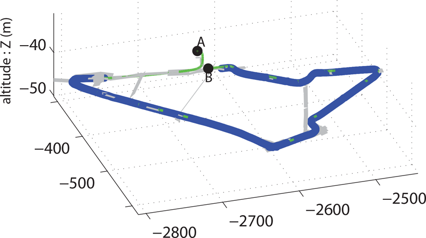
It has been experimentally found that at least 30 matched points are necessary to give an admissible result;
The succession of the estimates of the poses must be compatible with the kinematical model (3), which can be tested with a simple Mahalanobis test;
Figure 9(b) illustrates another problem tied to the convergence of the optimizations involved in the localization process. In this part of the trajectory, it has been found that the localization algorithm takes too much time in processing one image. Some frames are thus dropped and it yields discontinuities in the estimated trajectory.

Visual localization (blue) - reference trajectory (green) - illustration of some visual localization problems
In conclusion, the visual based localization generally gives results that are sufficiently accurate to locate the vehicle at the lane size but it is subject to failures that should be monitored. When a fault is detected, it is convenient to trigger another method based upon different data and principles to update the localization estimate. We propose in the sequel to use a MATGO method that takes advantage from the available geographic digital maps, odometric and GNSS sensors commonly installed on vehicles.

Example of the current video frame and its closest key frame for the Figure 9(a) case
This section presents the principles of a method that combines odometry (Section 5.1), GNSS data in tight coupling (Section 5.2) and fusion with geometric map data (Section 5.3). The underlying principles of this method are different from those of the visual-based method. This is an argument for the integrity of the collaboration of the two methods.
Odometric Update of the Localization
Each time odometric measurements are available, a new prediction is performed by using the state propagation equation (3) [32].
Tight coupling Satellite-based Localization
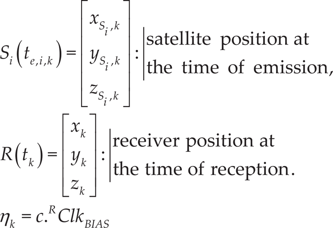
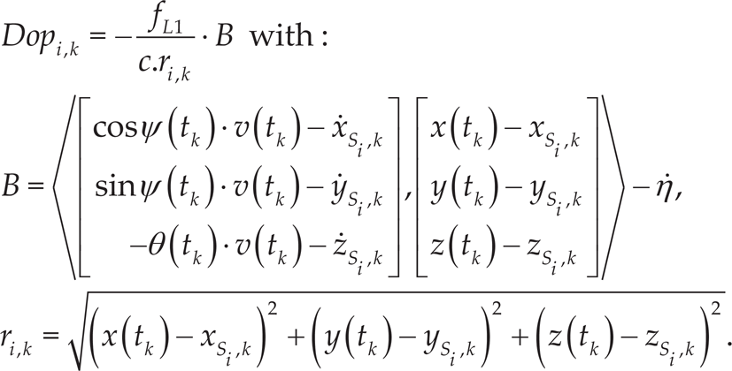
When some GPS data - either pseudo-range or Doppler data - are available, an a posteriori update is realized in the EKF algorithm. The associated state model is

where
In order to use the state space model (3), GPS measurements are expressed in terms of the state components.
Concerning the
where R Clk BIAS is the receiver clock bias. These notations give the corrected pseudo-range measurement,

The first part of the observation equation is given by:

Concerning the

This relative speed is linked with the frequency shift via the classical Doppler equation where fL1 = 1575.42[MHz] is the frequency of the L1 carrier of the GPS signal:

The Doppler measurement is this frequency shift f
rec
- fL1. Taking into account the drift of the receiver clock bias
The odometric/GPS data-fusion process has been implemented by using an EKF. At any time t
k
where some information becomes available, the method updates an estimate

Note that the time instants of the odometry and GPS signals are completely decorrelated, which implies that: i) when odometric data appear, the predictive part of the EKF is processed, and ii) when admissible GPS data occur, the updating part of the EKF is processed.

Updating the ellipsoidal confidence domain by using a road segment
The use of the geographical data is based upon the assumption that the vehicle moves on a road with a known geometric specification stored in the GIS. Usually, a road network is represented with set of connected polylines. Taking an estimation of the road width and the altitude inaccuracy of the map into account, each line segment forming the road can be extended to a box (Figure 12). In this study, we consider that the set of all these boxes represents the set of all acceptable positions of the car. This set can be used to constrain the ellipsoidal confidence domain obtained with tight-coupled GPS (Figure 11). For this, two steps are needed: i) to select the box in which the vehicle is assumed to be, and ii) an ellipsoidal confidence domain update using this knowledge.
Map Matching: Selection of a Road Segment
The initial selection of the road segments on which the vehicle may be located is done by testing the intersection of their bounding boxes with an ellipsoidal confidence domain obtained with tight-coupled GPS. If more than one box is found, the index i of the road segment on which the vehicle is supposed to be is selected by minimizing a linear combination of: 1) the 3D distance between the (x,y,z) projection of the centre of the a priori ellipsoid and the segment
Localization Update from the Knowledge of the Patch
Consider a formal expression of the box R
i
(Figure 12) - tt is included in a plane whose unit normal is
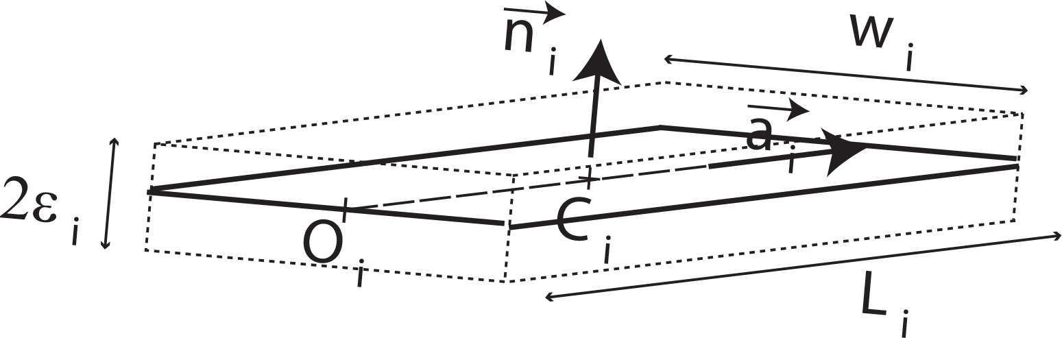
The i th box of the drivable area

Taking into account the height inaccuracy ε h i = 25 cm of the GIS, the first equation of (12) is better described by the inequality

The box R i is thus defined by three double inequalities that are linear in (x,y,z) and thus linear in q (1). Each inequality defines a band in the configuration space; for instance, the band (13) is the space between the two planes:

As illustrated in Figure 11, updating the set of acceptable positions of the vehicle consists of finding a set including the intersection of the a priori ellipsoidal confidence domain with the box R i . Since the pioneering work of Schweppe [33], ellipsoidal set membership estimation has proposed algorithms that compute an a posteriori ellipsoid containing the intersection of a band with an a priori ellipsoid. Among them, we have selected the optimum volume ellipsoid (OVE) algorithm [34]. Combining an a priori estimation with the knowledge of the box R i is then done by applying the OVE algorithm three times with each linear inequality of (12 and 13), the result being an ellipsoidal domain (11).
This step completes the method [35].
Recall that the time instants of the odometry and GPS signals are completely decorrelated and that the map-matching can be done on demand. Since each data flow has its own time-scale, their asynchronous processing can be represented by a state chart (Figure 13) where all the tasks have their own trigger and update the common ellipsoidal domain (11) specified by (

MATCGO state chart: three asynchronous tasks updating a common ellipsoidal domain
A 3D view of the results is displayed in Figure 14. Their accuracy is quantified by the cumulative distribution function of the absolute 3D error (Figure 15). It is not sufficient to localize the vehicle at the lane level as is the case for visual localization (Figure7).
In conclusion, although the use of map-aiding enhanced the accuracy of the 3D localization, it is not sufficient to localize the vehicle at the lane-level. On the other hand, this estimation is continuous and reliable.

MATCGO (blue) - Compared to the localization obtained by the LANDINS reference trajectory measurement (green) - Modelization of the road network in light grey
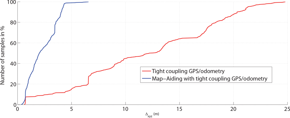
MATCGO - Cumulative distribution function of the absolute error in 3D
In order to deal with the visual localization problems reported in Figure 9, three criteria are checked prior to any visual estimation:
The number of landmarks: the localization is valid when there are at least 30 inliers. This corresponds to a lack of data in Figure 9(a);
Continuity: the new localization must be coherent with the previous one. It is checked by a Mahalanobis distance test that prevents the use of discontinuous estimates shown in Figure 9(a);
Computation time: this must be less than 200 ms. It detects the discontinuities in Figure 9(b).
Assuming that the MATCGO localization algorithm always updates a localization estimate
When visual localization is available (i.e., the database exists and the method is not lost) and validates some measurement criteria, the collaboration returns the estimate of this method;
Otherwise, the collaboration returns an estimate of the 3D MATCGO localization algorithm (Section 5.3).

Collaboration state chart
Both methods deliver an ellipsoidal confidence domain (11). The estimated vehicle configuration is the centre of this ellipsoid associated with a positive definite matrix defining the ellipsoid.
Switching is simply performed by:
When the visual localization does not validate one of the three measurement criteria, the MATCGO localization is used after having been updated by the last “good” visual localization in order to keep continuity;
When the visual localization again validates the three measurement criteria, the detection threshold is temporarily increased to ensure the stability of the solution.
The 2D and 3D results (Figure 17 and 18) illustrate the interest of the collaboration. Indeed, the absence of a database and the visual localization problems have been compensated for. Moreover, except during the first switch, continuity is maintained.

Collaboration localization (blue for visual, red for MATCGO) - Compared to the localization obtained by the LANDINS reference trajectory measurement (green)

Collaboration localization (blue for visual, red for MATCGO) - Compared to the localization obtained by the LANDINS reference trajectory measurement (green) - Modelization of the road network in light grey
Figure 19, where the cumulative distribution functions of the absolute error in 3D for the three methods are plotted, clearly demonstrates the limits of each individual method and the benefit of the collaboration. The visual localization is accurate but cannot protect from discontinuity or incoherence, whereas the MATCGO localization is not precise enough when used alone but it provides both reliable confidence tests of the estimates and a window to the database of visual landmarks to quickly initialize the visual method. This collaboration adds integrity to the accuracy of the visual-based localization and gives a continuous evolution of the accuracy.

Cumulative distribution function of the absolute error in 3D
This paper has demonstrated the interest of the collaboration between two localization methodologies based upon different data sources to supervise the displacement missions of a vehicle in dense urban environments. One method is vision-based and uses a database of visual landmarks acquired in a preliminary learning phase. The other method combines odometry with data from a digital map of the road network together with data from satellites of a GNSS when it is available, that is to say rarely in environments with poor satellites visibility. The geometry of the road network and the visual landmarks are defined in the same coordinates and constitute two layers of the GIS, used both for planning and execution control purposes. Both methods define the results of a localization as a feasible ellipsoidal domain in the configuration space.
Vision-based localization has been shown to be sufficiently accurate to locate the vehicle at the lane-level whereas the accuracy of the MATCGO method is not so good. On the other hand, the MATCGO method is obviously more reliable since: i) the databases it uses are already available almost everywhere, and ii) due to the tight fusion algorithm, it is robust against long periods of poor satellite visibility.
The vision-based method may fail in certain uncommon situations. This can be the case not only where there are not enough visual landmarks but also when the optimization algorithm does not converge in due time, as well as in special cases where the result of the visual localization is discontinuous since its principle does not guarantee the unicity of the solution. In this case, the MATCGO method running in parallel helps to detect this discontinuity and maintain a localization, which is important since the visual database of the GIS will certainly not be immediately available everywhere in the near future. In addition, the continuous result of the MATCGO method speeds up the initialization of the visual method where it can be used by restricting the numbers of landmarks in the database to be matched. From a technical viewpoint: 1) it has been useful to design a 3D kinematical model because the images are very sensitive to the variations of the axis of the camera, 2) the fact that the visual landmarks are referenced in the coordinates of the GIS has received a careful attention, which is important since the visual control of the trajectory must be achieved within the same reference frame as the lane marks, side walks and pedestrian crossings that materialize on the planned path.
The method was implemented in a full-scale experiment of 4 km in the centre of Paris which is a typical dense environment.
Footnotes
8.
This work was funded within the framework of the CityVIP project under the reference project ANR-07-TSFA-013-01. We thank particularly IFSTTAR for their help in collecting data on their “VERT” experimental vehicle and the MATIS laboratory of IGN for their geographical databases.
1
NMEA GGA: latitude, longitude and altitude computed by the receiver from the raw data with its own algorithm.
2
The positive definite matrix P
k
may be linked with a validity domain of a Gaussian estimation