Sage Journals: Discover world-class research

Abstract

To improve the real-time performance and detection rate of a Lane Detection and Reconstruction (LDR) system, an extended-search-based lane detection method and a Bézier curve-based lane reconstruction algorithm are proposed in this paper. The extended-search-based lane detection method is designed to search boundary blocks from the initial position, in an upwards direction and along the lane, with small search areas including continuous search, discontinuous search and bending search in order to detect different lane boundaries. The Bézier curve-based lane reconstruction algorithm is employed to describe a wide range of lane boundary forms with comparatively simple expressions. In addition, two Bézier curves are adopted to reconstruct the lanes' outer boundaries with large curvature variation. The lane detection and reconstruction algorithm — including initial-blocks' determining, extended search, binarization processing and lane boundaries' fitting in different scenarios — is verified in road tests. The results show that this algorithm is robust against different shadows and illumination variations; the average processing time per frame is 13 ms. Significantly, it presents an 88.6% high-detection rate on curved lanes with large or variable curvatures, where the accident rate is higher than that of straight lanes.

Keywords

Lane Detection Lane Reconstruction Extended Search Bézier Curve Intelligent Vehicle

1. Introduction

In order to improve traffic safety, the United States began research on intelligent vehicles in the 1990s [1]. Since then, ADASs (Advanced Driver Assistance Systems) have been attracting more and more attention as an important part of this field.

Over nearly two decades, much research has focused on detecting the driving environment information with a forward-looking camera installed on the front of a vehicle. The LDR system extracts lane boundaries from the images and defines them with a proper curve model, which should have high real-time performance and detection rate. The research into LDR systems experiences some difficulties, such as:

How to avoid the interference caused by shadows from roadside trees or buildings;

How to reduce misjudgements due to obstacles in the images;

How to maintain robustness in varying illumination conditions;

How to adapt to different lane shapes and curvatures;

How to accurately detect and reconstruct lanes in real time.

Many lane features have been used in detection research, such as colour [2], width [3] and texture [4]; however, some of those features may reduce the robustness of the method because of their sensitivity to illumination. In [5] and [6], the methods used for lane detection at night-time partially solve the problem of light sensitivity. The input images were usually converted to edge images by using Sobel [7], Canny [8] or dark-light-dark transition [3, 9]. However, some lane boundaries could not be extracted in the edge images due to the large or dense shadows on the road, and some useful boundary information would be lost. Borkar and Xu put forward a method of inverse perspective mapping (IPM) to convert the original image to a bird's-eye view image before further detection [10,11]. Since the IPM processing is done on the entire image and the lane markings only occupy a very small area in the image, most of the calculation efforts are wasted. Wu [12] used local adaptive threshold in blocks and edge-compensation masking to get boundary edge images. This method is effective against shadow interference. However, the fitting models of the straight-line and parabola they used could be better suited to a curve with a small curvature.

Straight-line models have been used widely in the literature, such as those used in Hough Transform (HT) [13] and its modified forms. Straight-line models work well on the straight road without navigational text and arrows, but the detection rate will deteriorate if they are used on curved road. Deformable lane models work well on curved roads, forms such as the piece-wise linear [14], clothoid [15] and hyperbola [16]. Though applicable to lanes with more complicated shapes, deformable models are susceptible to noise and require longer processing times. In the path-planning field, the Bézier curve has been widely used with a simple mathematical definition and flexible shapes [17], Han [18] designed an anti-collision path planner using a fourth-order Bézier curve. They used the position, velocity direction and curvature parameters of the start and end points to calculate the other control points. However, in our system the above parameters are unknown in advance. Hilario [19] and Kawabata [20] used fifth- and eighth-order Bézier curves to generate paths, but the higher the Bezier curve, the heavier the calculation. Clothoids and rational Bézier curve-based path planning have also been researched in recent years [21, 22]. Nevertheless, the numbers of orders are high and the calculations of control points are complex. Since the shapes of lanes are not normally very complex, we tend to use lower Bézier curves to reduce the complexity of the algorithm.

Proposed in this paper is an extended-search-based lane detection method. Intended for enhancement of the real-time performance and the rate of lane detection, compared with other methods, a merit of this method of extended search is a high degree of search efficiency by exploiting the continuity and smooth transitions of lane markings in the images. Searching lane boundary blocks using extended search can adapt to both straight and curve lanes with small search areas. Additionally, we designed a lane reconstruction algorithm by using a second-order Bézier curve. A metric to measure the quality of the lane reconstruction is also presented. When the value is below the threshold, the boundary will be fitted by two connecting second-order Bézier curves, which could improve the reconstruction quality.

This paper is organized as follows: Section 2 shows the system configuration of the LDR. Section 3 describes the lane-detection method, mainly gradient feature presentation and extended search processing. Pane reconstruction focusing on boundary models and fitting is discussed in Section 4. Experimental results and comparison are given in Section 5. Finally, conclusions are provided in Section 6.

2. System configuration of LDR

The architecture of the intelligent vehicle is shown in Figure 1(a). The camera used for the LDR system is installed on the support behind the rear-view mirror inside the vehicle, as illustrated in Figure 1(b). The grey images captured by the camera are transmitted to the central control computer. The LDR system in the computer then processes the images to extract the two lane boundaries for the vehicle.

Figure 1.

System configuration of the intelligent vehicle: (a) overview of a simple intelligent vehicle system, (b) system scheme illustration and (c) camera projection illustration

The flowchart of the LDR algorithm is shown in Figure 2. There are two parts to the algorithm: lane detection and lane reconstruction. Lane detection involves searching boundary blocks from the initial position upwards along the lane direction. Lane reconstruction fits boundaries with a Bézier curve.

Figure 2.

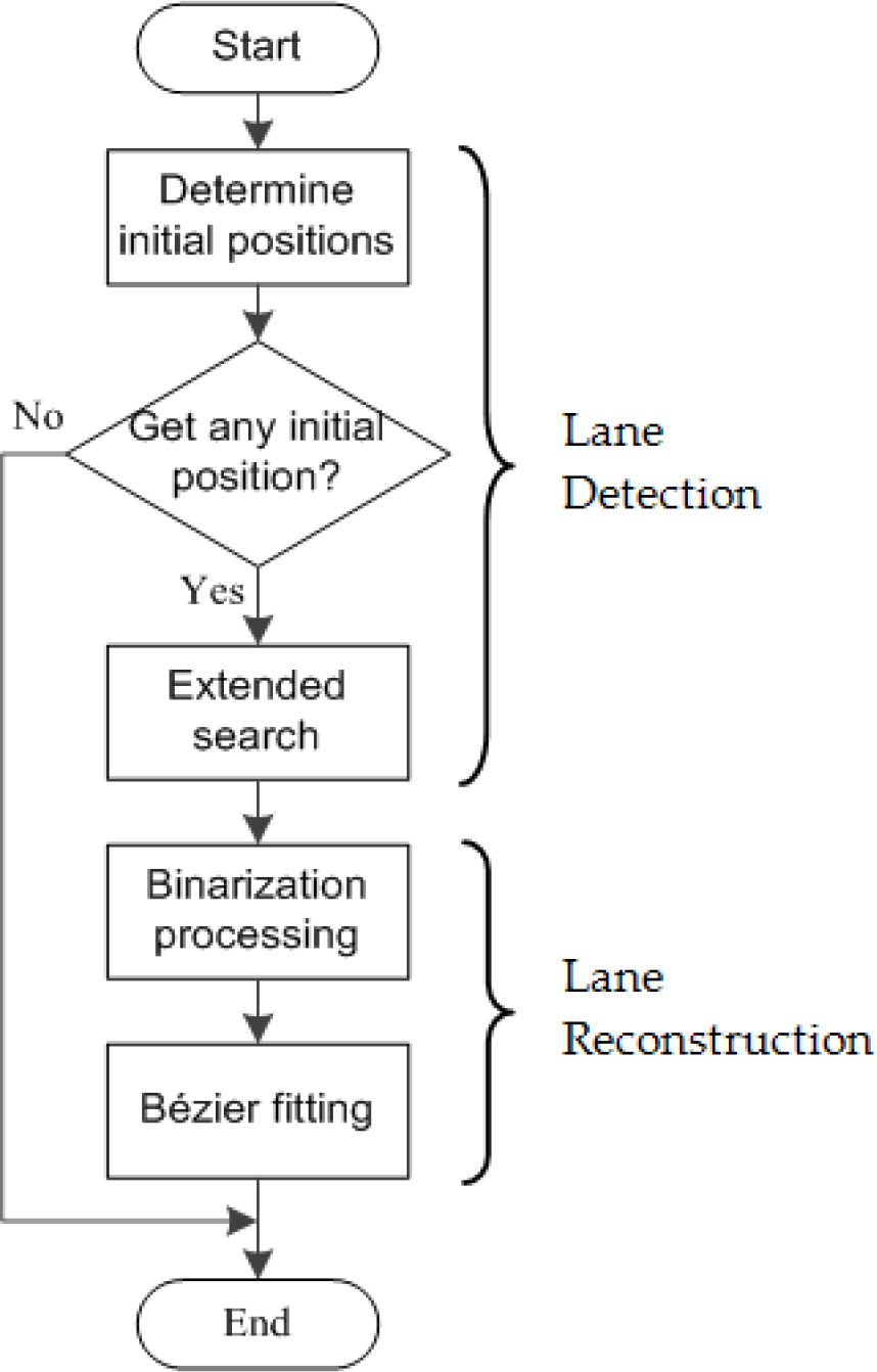
Flowchart of the LDR algorithm

3. Lane detection algorithm

3.1 Gradient feature of lane boundary

In general, the pitching angle α of the camera is small and the road in the images occupies only a part of the whole screen in the y−direction (see Figure 3). The heights h and α change very little after the camera is fixed on the support. Therefore, the maximum processing scope y₀ in the y-direction could be set in advance according to the installation position of the camera. In this paper, we set y₀ = 150.

This paper focuses on structural roads with relatively clear road-lane markings. There are obvious grey level changes from lane-boundary markings to the pavement, which is not influenced by shadows, illumination or the colour of lane markings. When intercepting image blocks of the proper size at the proper position, a distinct gradient feature exists in them (see Figure 3(a) and 3(b)). In addition, each of the blocks is approximately divided into two triangles by the lane boundary (assuming that the vehicle is driving in one lane and is not in the state of lane changing).

Figure 3.

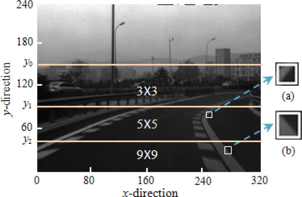
Image coordinates and processing-scope configuration; (a) and (b) are obvious gradient features

The farther the distance from the camera, the narrower the width-lane markings are in the images. Therefore, the blocks LxL that are used for calculating gradient feature values should have different sizes at different distances. Lots of experiments and simulation results show that dividing the processing area into three parts with different block sizes in the y-direction has better effects than other methods. They are shown in Figure 3: [0 y₂], [y₂y₁] and [y₁y₀] (in this paper y₂ = 45, y₁ = 90), and the sizes of LxL = 9 × 9, 5 × 5 and 3 × 3, respectively. Additionally, when the lane is curved, the gradient directions of blocks will always change on one side of the lane boundary (see Figure 3(a) and 3(b) for examples). Therefore, it is necessary to design more than one set of masks to calculate the gradient eigenvalues T of the blocks, as shown in Figure 4 (c = −2/(L²−L), d = −2/(L²−L)). The second set of masks ② and ④ are used in the bending search of the extended search; masks ① and ③ are used in other situations. If the eigenvalue T is greater than the threshold T₀ the block satisfies the gradient feature and it may contain a lane boundary. In this paper, we set T₀=15 during the day and T₀=10 at night from empirical data.

Figure 4.

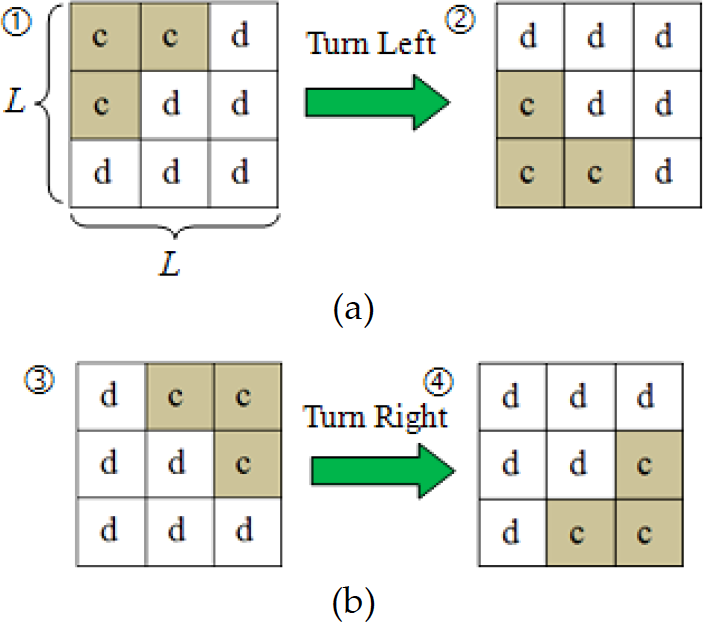
Two sets of masks for the left- and right-hand boundaries: (a) masks for the left-hand boundary, (b) masks for the right-hand boundary

The real-time performance of a lane detection algorithm largely depends on search method efficiency. If we could control search areas around the lane boundaries, and search blocks from an initial position upwards along the lane direction as shown in Figure 5, then the real-time performance and detection rate would be improved. Following this idea, we firstly determined the initial blocks.

Figure 5.

Illustrations of a proposed search method of lane detection

3.2 Determining the initial position

The initial blocks are the lowest position of the left- and right-hand boundaries, which are the starting blocks for the extended search. To reduce the interference of other road signs, the searching areas of the left- and right-hand boundaries of the initial blocks are shown in Figure 6 (x_L = 106, x_R = 213, y_LR = 100 in this paper). The areas can satisfy most of the conditions when the vehicle is driving in the lane throughout the experiment.

Figure 6.

Illustration of the lane's initial block searching areas

To avoid the interference from the marks on the road, such as driving arrows, we stipulated that in getting the initial block condition, an additional two continuous blocks were found in continuous searching. The searching order was also designed to reduce computing times. Firstly, the block that has the maximum eigenvalue at the bottom of the searching area is searched (see the dotted arrow in Figure 6). Then it is checked to see whether it meets the above condition. If not, search the outer-most position (see the solid arrow). If the initial block still cannot be found, search the block in the entire searching area from inside to outside, and bottom to up. The result is shown in Figure 7.

Figure 7.

Result of determining the initial blocks

3.3 Extended search

Extended search is a searching method covering small searching areas, which searches blocks one by one, upwards from the initial block along the outer boundaries. Firstly, set the potential area for the next block based on the searched adjacent blocks. Then find a block that has the maximum gradient eigenvalue in it. If the eigenvalue is greater than threshold T₀, the block is the boundary block. Otherwise, update the potential area and continue searching.

Lanes have various forms, such as straight or curved, continuous or discontinuous. Figure 8 shows four common forms of left-hand boundary. Obviously, it is hard to design only one method of setting the potential area for the different lane forms. Therefore, we designed continuous search, bending search and discontinuous search methods to adapt to different forms.

Figure 8.

Four common lane forms of left-hand boundary and their corresponding search method

Figure 9.

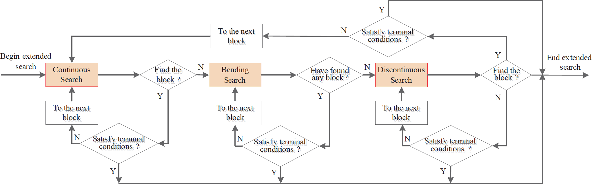
Flowchart of extended search

Figure 9 shows the flowchart of the extended search. At the beginning of the extended search, the continuous search is used. If it does not find the boundary block, it will go to the bending search. If still does not get it, the boundary at this position is probably discontinuous. In that case, use discontinuous search and once a boundary block is found, go back to continuous search.

3.3.1 Continuous search

In continuous search, gradient eigenvalues of blocks are calculated by mask ① or ③ and potential areas are set based on the coordinate change of two adjacent searched blocks; that is assuming we have searched n blocks in a left-hand boundary that is represented by red frames in Figure 10. The coordinates of the outside lowest points of each block are P_i(x_i, y_i)(i=1, 2, ⋯, n). The search scope of (n+1)th block's outside lowest point P_n+1(x_n+1, y_n+1) is designed as:

\begin{matrix} y_{n + 1} = y_{n} + L \\ x_{n + 1} \in [x_{n} - s_{1}, x_{n} + (x_{n} - x_{n - 1}) + s_{2}] \end{matrix}

(1)

where L is the size of the nth block and s₁ and s₂ represent the left and right offset. In general, x_i is greater than x_i−1 in the situation of continuous search. Therefore, s₁ should be set smaller than s₂ to avoid lane boundaries going beyond the search areas.

Similarly, for the right-hand boundary, the search scope of the (n+1)th block's outside lowest point P′_n+1 is designed as:

\begin{matrix} {y^{'}}_{n + 1} = {y^{'}}_{n} + L \\ {x^{'}}_{n + 1} \in [{x^{'}}_{n} + ({x^{'}}_{n} - {x^{'}}_{n - 1}) - s_{2}, {x^{'}}_{n} + s_{1}] \end{matrix}

(2)

Calculate each block in the potential areas using the first set of masks and find the maximum eigenvalue block. If the eigenvalue is greater than T0, it will continue to the next block. In Figure 11, the white squares in the potential areas are the search results of completing a continuous search on each boundary, once.

Figure 10.

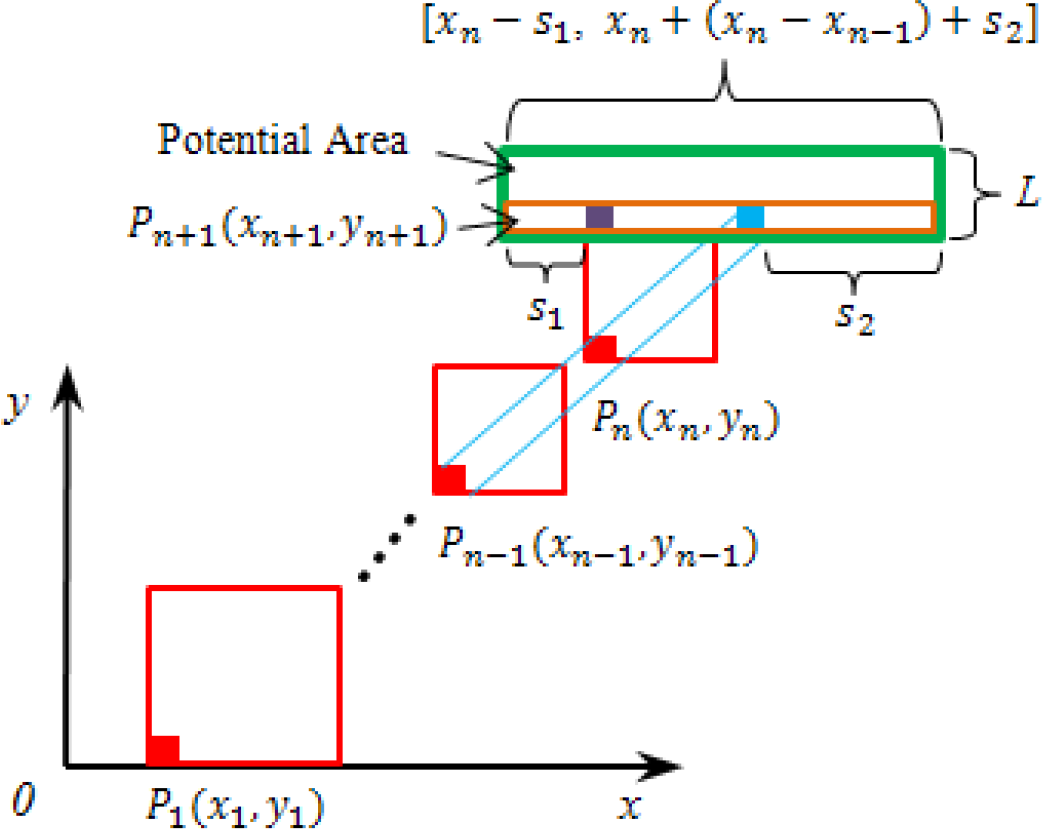
Illustration of setting the potential area for the left-hand boundary in a continuous search

Exceptionally, point P₀ does not exist when searching the second block in determining initial blocks. The search scope of point P₂ is set according to experimental data: y₂=y₁ + L, x₂ ∊ [x₁, x₁ + 20]; such that point P′_n+1 is: y′₂ = y′₁ + L, x′₂ ∊ x′₁ −20, x′₁].

Figure 11.

The results of using continuous search once on each boundary

3.3.2 Bending search

The blocks of lane boundaries under continuous search tend to extend to the middle of the image. However, the lane boundary trend changes to an outwards direction after turning. Therefore, bending search is different from continuous search in setting the potential area and using mask ③ or ④ to calculate eigenvalue T.

The search scopes of the outside lowest points in bending search are designed as:

Points on the left-hand boundary P_n+1:

\begin{matrix} y_{n + 1} = y_{n} + L \\ x_{n + 1} \in [x_{n} + (x_{n} - x_{n - 1}) - s_{2}, x_{n} + s_{1}] \end{matrix}

(3)

Points on the right-hand boundary P′_n+1:

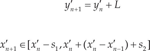
\begin{matrix} {y^{'}}_{n + 1} = {y^{'}}_{n} + L \\ {x^{'}}_{n + 1} \in [{x^{'}}_{n} - s_{1}, {x^{'}}_{n} + ({x^{'}}_{n} - {x^{'}}_{n - 1}) + s_{2}] \end{matrix}

(4)

Figure 12 is the resulting image of using bending search once on the right-hand boundary. Since the lane generally has only one turn, the bending search will keep working until it comes to the terminal conditions. The system will always search the left lane first, and there is only one side boundary that bends on a curved lane; therefore, use of bending search on the right-hand boundary will be cancelled automatically when the left lane is confirmed as including a turn.

Figure 12.

The result of using bending search once for a right-hand boundary

3.3.3 Discontinuous search

In some cases, the lane boundaries may be discontinuous or obscured by obstacles. By analysing the smoothness of lane markings, the distance x_d on the x-direction - from the starting point of the lane's outer boundary after the break to the straight line, through the starting and ending points of the lane before the break - is found to be relatively small (see Figure 13).

Figure 13.

The small distance on the x-direction, from the starting point after the break to the straight line that passes through the starting and ending points before breaks

Taking advantage of the above features and the n outside the lowest detected points P_i(x_i, y_i) (i=1, 2, ⋯, n), the potential area of discontinuous search is set as:

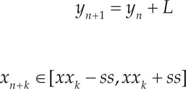
\begin{matrix} y_{n + 1} = y_{n} + L \\ x_{n + k} \in [x x_{k} - s s, x x_{k} + s s] \end{matrix}

(5)

where k represents the number of blocks from the break upward (k = 1,2, ⋯, 10), L represents the size of the corresponding block y_n+k−1, ss represents the left and right offset and xx_k represents the x−coordinate of the point on the straight line through the starting point P_a(x_a, y_a) and ending point P_n(x_n, y_n), when y = y_n+k.

x x_{k} = (x_{n} - x_{a}) / (y_{n} - y_{a}) + x_{a}

(6)

Figure 14.

Illustration of the setting potential area for the left-hand boundary in discontinuous search

The result of discontinuous search performed once for the right-hand boundary is shown in Figure 15.

Figure 15.

The result of the discontinuous search

3.3.4 Terminal conditions

Considering the limitations of the processing area, the general trend of boundaries and the non-intersection of left-and right-hand boundaries, we designed the terminal conditions notifying the computer that the search had finished as follows:

The potential area exceeds the maximum processing area;

If one boundary block was found in bending search, it means that the boundary trend has changed. Because curved lane boundaries are normally continuous, the extended search will not end until it cannot find a block. Some curved lane boundaries with small curvatures may also be discontinuous, but the distance between the bending position and the host vehicle is large enough to meet the need of the LDR system;

k > 10 in discontinuous search;

The potential area includes the left-hand side of the endpoint's approximate tangent of the left-hand boundary when searching for the right-hand boundary blocks (see Figure 16).

Figure 16.

Illustration of the fourth limiting condition for right-hand boundary blocks

Figure 17.

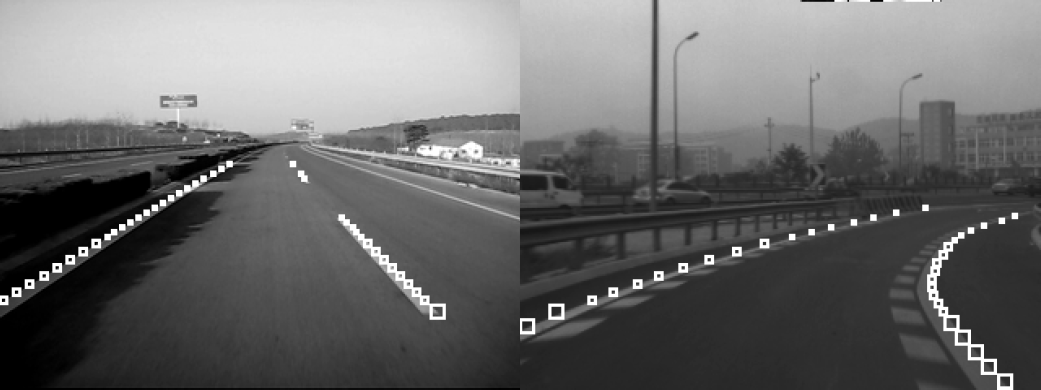
Illustration of the fourth limiting condition for right-hand boundary blocks

Once one of the above four conditions is satisfied, the search for boundary blocks will end. Figure 17 shows the results of an extended search of left- and right-hand boundary blocks.

4. Lane reconstruction algorithm

4.1 Lane boundary model

Lane reconstruction's aim is to fit the boundaries accurately by using a lane model. An n^th Bézier curve can be represented as:

p (t) = \sum_{j = 0}^{n} b_{j} B_{j, n} (t)

(7)

where b_j is the control points and t ∊ [0,1]; B_j,n(t) is the Bernstein basis polynomial given by $B_{j, n} (t) = {\begin{matrix} C_{n}^{j} t^{j} {(1 - t)}^{n - j}, \\ 0, \end{matrix} \begin{matrix} i f \begin{matrix} \end{matrix} j = 0, 1, \dots, n \\ o t h e r s \end{matrix}$ .

A conic Bézier curve is determined by just three control points, as shown in Figure 18(a). The control point b₀ and b₂ are the start- and end-points of the curve, respectively, and the intermediate control point b₁ is the intersection point of two tangents from the points b₀ and b₂. Once b₀ and b₂ are determined, the curve shape just depends on b₁.

In general, lane boundaries can be reconstructed accurately with one conic Bézier curve. However, when the lane curvature varies, the fitting quality will deteriorate. In this case, control points should be added by using one cubic Bézier curve or two conic Bézier curves. We chose two conic Bézier curves as shown in Figure 18(b) because both of the two intermediate control points b₁ and b₃ have strong constraints, creating a wide shape range for lane boundaries.

4.2 Lane boundary fitting

In order to extract edge pixels, the method of Maximum Classes Square Error (named Otsu [23]) is used in every searched block, as shown in Figure 19. In these blocks, the lowest points Q_i(x_i y_i)(1≤i≤m) of the lane's outer boundaries can be easily obtained (m is the number of a lane boundary's blocks). When using only one Bézier curve to fit the boundary, Q₁ is the starting control points, Q_st and Q_m is the ending control points Q_en, respectively. Therefore, we just need to find the optimum intermediate control points to obtain the optimum Bézier curves, given that the intermediate control point is the intersection point of two tangents from the starting and ending points.

Figure 18.

Lane boundary models for different curvatures: (a) one conic Bézier curve for a left-lane boundary, (b) two conic Bézier curves for a variable curvature lane boundary

Figure 19.

Adaptive binarization processing for each block: (a) straight lane, (b) curved lane

Though these tangents are indefinite, we can connect starting control point Q_st and its next point Q_st+1 as the approximate tangent of Q_st, and connect the ending control points Q_en and Q_en−-1 as the approximate tangent of Q_en(1≤sten≤m). The intersection point of the two approximate tangents is close to the real intermediate control point; therefore, the potential area of the intermediate control point can be divided based on the intersection point (see the white rectangles in Figure 20 and the size is 20 × 20 in this paper).

Figure 20.

Potential areas for intermediate control points

Every point in the potential area can construct a Bézier curve with the starting and ending control points. Due to the binarization processing of each block, the difference in grey value between the two sides of the optimal Bézier curve should be the largest. Therefore, an objective function is designed as:

F (t) = \sum_{t = 0}^{1} (g_{t} - g g_{t})

(8)

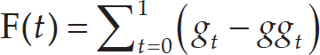
where g_t is the pixel value of the point p_t on the curve and gg_t is the pixel value of the outer adjacent point of p_t.

Additionally, the lane is considered to be straight if the intersection of approximation tangents does not exist. The line connecting the starting and ending control points is determined as the optimal curve.

Figure 21.

Fitting result by using one Bézier curve

4.3 Quality metric and improvement

In this paper, we also design a metric to measure the quality of the lane reconstruction, as shown in Equation (9).

R = \frac{\sum_{i = 1}^{m} | \bar{S_{i}} - \bar{V_{i}} |}{255 m}

(9)

where R is the metric value, R ∊ [0, 1] and $\bar{S_{i}}$ is the average of the sum of the pixels' values, which are on the inner side of the Bézier curve in a statistical block. They are lane-marking pixels, if the reconstruction quality is high enough. In addition, $\bar{V_{i}}$ is the average of the sum of the remaining pixels' values in the block and m is the number of statistical blocks. Because a discontinuous boundary may exist, not all of the blocks that are determined by the Bézier curve are calculated. Statistical blocks only include the blocks that should be on the lane marking, according to the extended search result.

In Figure 21, both left-hand boundaries are of high reconstruction quality. Their metric values are 0.87 and 0.76, as shown in Table 1. However, the right-hand boundary in Figure 21(b) is of low quality and the metric value is only 0.24. It should be fitted again using two Bézier curves so that the metric value could also be used to determine whether two Bézier curves are needed to fit the boundary.

We set a threshold: R₁. If RR₁, the boundary will be fitted with two continuous Bézier curves to improve the reconstruction quality (R₁=0.4 in this paper).

The intersection point is the ending point and starting point of the first and second Bézier curves, respectively. This point should be around the position where the most obvious change occurs. Adjacent points Q_i and Q_i+1 are connected by straight lines. The slope changes of those lines can roughly reflect the degrees of lane bend and the position where the most obvious change occurs. Therefore, first calculate the slopes t_k(1k≤m−1) of the straight lines using Equation (10). Then calculate the slope difference τ_kk(1≤kk≤m−2) between adjacent straight lines using Equation (11) to find the maximum τ_mm among τ_kk, and Q_mm+1 is the intersection point. Figure 22 shows the improved reconstruction quality, when compared to that of Figure 21(b), by using two Bézier curves.

t_{k} = (x_{i + 1} - x_{i}) / (y_{i + 1} - y_{i})

(10)

τ_{k k} = | t_{k + 1} - t_{k} |

(11)

Table 1.

R value of the fitting result in Figure 21(a) and (b)

Boundaries	Figure 21(a)		Figure 21(b)
Boundaries	Left-hand boundary	Right-hand boundary	Left-hand boundary	Right-hand boundary
R	0.87	0.58	0.76	0.24

Figure 22.

Fitting the right-hand boundary with two Bézier curves

5. Experiment results and analyses

5.1 Complex scenarios

The LDR system has been verified in the real road images. The camera was mounted at height h=1.35m and pitch angle α=5°. The image resolution was 320 × 240. The real road images used for testing the database were captured on highways or urban roads in and around Beijing under different conditions of illumination, shapes of shadows and curvatures. The speed of the vehicle was from 30 km/h to 60 km/h. Parts of results are shown as follows:

The results of the sequencing image with different shapes of shadows and obstacles are shown in Figure 23.

The image sequences were recorded on an urban road in Beijing. There are many buildings and trees on both sides, cars driving on the road, as well as overpasses going across the road. In this case, the driving environment is relatively complex.

The results show that the algorithm introduced in this paper could adapt to the environment even if there are shadows on the road. Additionally, extended search could also avoid interference from obstacles outside the searching areas. Take Frame 085, for example; there is a driving direction arrow on the road's centre, but it could still work well because the arrow is outside the searching areas. Gradient features of the lane boundaries are also effective under the interference of shadows. Adaptive binarization processing for each block makes a large contribution to obtaining points of lane boundaries accurately. The total number of frames in this case is 1,308, of which 228 images fail the test (include missed and incorrect detection). The detection rate is 82.6%. The main reason for failure is the interference of vehicles that are close to the lane boundaries, as in Frame 253.

The image sequences and the search results tested on the curved road are shown in Figure 24.

These image sequences display a case of driving from a straight lane to a curved lane, which usually occurs in a merging lane. The results show that the boundaries' model and fitting method could adapt to both straight and curved lanes. The boundary with a larger curvature change (such as the right-hand boundary in Frame 164) is well fitted with two Bézier curves. The total number of frames in this case is 740, of which 84 failed the detection (include missed and incorrect detection). Therefore, the detection rate is 88.6%.

The system was also tested under different levels of illumination, as shown in Figure 25.

The results show that this algorithm has good adaptability to varying levels of illumination, and that the gradient feature on lane boundaries always exists unless the light is too weak or too strong. Extended search does not only help avoid interference from shadows and obstacles, but also improves the real-time performance due to its narrow search areas. The average processing time is 13ms per frame. The programming environment is Windows XP, CPU 3.30 GHz, Visual Studio 2010 and openCV 2.4.4.

5.2 Comparison analyses

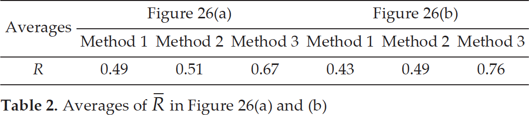
We used two other methods to process the two sets of image sequences shown above, in Section 5.1. Method 1 is a commonly used processing method, which first uses IPM to get a bird's-eye view, then gets edge images by using Sobel and finally uses HT and a width feature to get the lane boundaries. Method 2 is the algorithm that our team designed three years ago [24]. It uses an ant colony algorithm in boundary blocks' searching and a parabola model in boundary fitting. Method 3 is the approach that we discuss in this paper. We also measure the quality of the lane reconstruction results using Equation (9). The comparisons between these three methods are shown in Figure 26. In addition, Table 2 shows the averages of the metric value R in Figure 26(a) and (b).

Figure 23.

Results of the image sequences with different shapes of shadows and obstacles

Figure 24.

Sequence of resulting images with different curvatures

Table 2.

Averages of $\bar{R}$ in Figure 26(a) and (b)

Averages	Figure 26(a)			Figure 26(b)
Averages	Method 1	Method 2	Method 3	Method 1	Method 2	Method 3
R	0.49	0.51	0.67	0.43	0.49	0.76

Figure 25.

Resulting images under different illumination levels: (a) under strong light, (b) under dimmed light and (c) under road lights at night

In Figure 26(a), we can see that the metric value R and the detection rate of Method 1 and Method 3 are closed, in general. However, the reasons for their low quality are different. For Method 1, lane marking cannot be extracted after Canny when there are dense shadows. For Method 3, a large discontinuous space of the lane of the lane reduces the detection rate. In Figure 26(b), the straight-line parabola models are not flexible enough to reconstruct the large and variable curvature curves.

Figure 26.

Metric values of the boundaries: (a) in the first set of image sequences, (b) in the second set of image sequences

6. Conclusions

In this paper, we present an LDR system for the intelligent vehicle. The extended-search-based lane detection method makes full use of the smoothness and extensibility of lane boundaries. Th extended search algorithm includes continuous, discontinuous and bending searches, which are designed for detecting continuous, discontinuous and bending lane parts respectively. It can minimize the search areas greatly and adapt to most lane forms. A Bézier-curve-based lane reconstruction algorithm is effective for both straight and curved lanes, and variable curvature boundaries are reconstructed with two Bézier curves, which can improve the quality of reconstructions.

The LDR system was verified on real roads and the results show that the algorithm has strong robustness to varying illumination conditions and different shapes of shadows. It also has a high degree of fitting precision and real-time performance. On the other hand, after analysing the failing images, our future work will focus on reducing interference caused by other vehicles and unstructured roads.

Footnotes

7.

This research was supported by the Natural Science Fund of China (No. 51105021 and No.51405008), and Beijing Municipal Natural Science Foundation (No. 3133040).

References

and Lin

(2012) Member: Applying a Functional Neurofuzzy Network to Real-Time Lane Detection and Front-Vehicle Distance Measurement. IEEE Trans. Syst. Man. Cybern. Syst. 42: 577–589.

Wang

Zhang

(2004) Color-based Road Detection in Urban Traffic Scenes. IEEE Trans. Intell. Transp. Syst. 5: 309–318.

Marzotto

Zoratti

Bagni

. (2010) A Real-time Versatile Roadway Path Extraction and Tracking on an FPGA Platform. Comput. Vis. Image Understand. 114:1164–1179.

Zhang

Naqel

(1994) Texture-Based Segmentation of Road Images. IEEE International Conference on Intelligent Vehicles; 1994 Nov; Karlsruhe, Germany. pp. 260–265.

Borkar

Hayes

(2012) A Novel Lane Detection System with Efficient Ground Truth Generation. IEEE Trans. Intell. Transp. Syst. 13: 365–374.

Zhang

Zhong

(2009) Study on Lane Boundary Detection in Night Scene. IEEE Intelligent Vehicle Symposium; 2009; China. pp. 538–541.

Zheng

Cheng

(2004) Spring Robot: A Prototype Autonomous Vehicle and Its Algorithms for Lane Detection. IEEE Trans. Intell. Transp. Syst. 5: 300–308.

Wang

Cheng

Chen

(2010) Applying Fuzzy Method to Vision-Based Lane Detection and Departure Warning System. Expert Syst. Appl. 37: 113–126.

Jiang

Klette

Vaudrey

and Wang

(2011) Lane Detection and Tracking Using a New Lane Model and Distance Transform. Mach. Vision Appl. 22: 721–737.

10.

Borkar

Hayes

(2012) A Novel Lane Detection System with Efficient Ground Truth Generation. IEEE Trans. Intell. Transp. Syst. 13: 365–374.

11.

Wang

Zhou

Zheng

(2012) Real-Lime Lane Detection for Intelligent Vehicles Based on Monocular Vision. Proceeding of the 31st Chinese Control Conference; 2012; Hebei, China. pp. 7332–7337.

12.

Chang

and Lin

(2014) Lane-Mark Extraction for Automobiles under Complex Conditions. Pattern Recogn. 46: 2756–2767.

13.

Borkar

Hayes

Smith

Pankanti

(2009) A Layered Approach to Robust Lane Detection at Night. Computational Intelligence in Vehicles and Vehicular Systems; 2009; Nashville, TN. pp. 51–57.

14.

Lai

AHS

Yung

NHC

(2000) Lane Detection by Orientation and Length Discrimination. IEEE Trans. Syst. Man Cybern. B. 30: 539–548.

15.

Huh

Park

Hong

. (2005) Park: Development of a Vision-Based Lane Detection System Considering Configuration Aspects. Opt. Laser. Eng. 43:1193–1213.

16.

Khalifa

Assidiq

Hashim

(2009) Vision-Based Lane Detection for Autonomous Artificial Intelligent Vehicles. IEEE Int. Conf. Semantic Comput; 2009 Sept; Berkeley, CA, USA. pp. 636–641.

17.

Chen

Zhao

Mei

and Liang

(2013) Lane Change Path Planning Based on Piecewise Bezier Curve for Autonomous Vehicle. IEEE International Conference on Vehicular Electronics and Safety (ICVES); 2013; Dongguan, China. pp. 17–22.

18.

Han

Yashiro

Nejad

HTN

and Mita

(2010) Bézier Curve Based Path Planning for Autonomous Vehicle in Urban Environment. IEEE Intelligent Vehicles Symposium University of California; 2010; San Diego, CA, USA. pp. 1036–1042.

19.

Hilario

Montés

Mora

and Falcó

(2011) Real-Time Bézier Trajectory Deformation for Potential Fields Planning Methods; IEEE/RSJ International Conference on Intelligent Robots and Systems; 2011; San Francisco, CA, USA. pp. 1567–1572.

20.

Kawabata

Xue

and Zheng

(2013) A Path Generation Method for Automated Vehicles Based on Bezier Curve; IEEE/ASME International Conference on Advanced Intelligent Mechatronics (AIM); 2013; Wollongong Australia; pp. 991–996.

21.

Montés

Herraez

Armesto

and Tornero

(2008) Real-Lime Clothoid Approximation by Rational Bezier Curves. IEEE International Conference on Robotics and Automation; 2008; Pasadena, CA, USA. pp. 2246–2251.

22.

Brezak

and Petrovic

(2014) Real-Lime Approximation of Clothoids with Bounded Error for Path Planning Applications. IEEE L. Robot. 30: 507–515.

23.

Otsu

(1979) A Threshold Selection Method from Gray-Level Histogram. IEEE Trans. Syst. Man Cybern. 9: 62–66.

24.

Zhang

Huang

Liu

. (2011) Image Vehicle Motion Trajectory Prediction Method under Complex Environment. Chinese Journal of Mechanical Engineering. 47:16–24.

Extended-Search,Bézier Curve-Based Lane Detection and Reconstruction System for an Intelligent Vehicle

Abstract

Keywords

1. Introduction

2. System configuration of LDR

3.1 Gradient feature of lane boundary

4.1 Lane boundary model

5.1 Complex scenarios

5.2 Comparison analyses

Footnotes

7.

References