Sage Journals: Discover world-class research

Abstract

One of the most outstanding problems of our technical age is the heavy aerial pollution. There are several well-known methods [6, 10 –15] that exist for large-area pollution detection, but the measurement of the exact rate of pollution in smaller areas (e.g., industrial zones or disaster-affected areas of a few square kilometres), as well as the numerical expression of changes therein, remain an unsolved problem.

The main feature of the developed device is that it can provide exact measurements for a small area at low altitudes (under 500m AGL (Above Ground Level)), and it is also capable of periodical measurements between 0.0001–10 Hz. With the data analysis provided by the system, we can obtain immediate information about the pollution of the given area, as well as changes in pollution levels over time.

Keywords

Multi-rotor Aerial Pollution 3D Data Collection Autonomous Flight 3D Pollution Map

1. Introduction

The system (which consists of a carrier device, an on-board high-intelligence measurement system and a software program that is used to analyse the data) is capable of recording air parameters like humidity, temperature, dust, radiation, chemical pollution, etc., with exact geographical precision. During the processing of the measured data, the ground software obtains a 3D map that effectively illustrates the distribution of the pollution and, after multiple measurements, the spread direction and velocity of the pollution as well.

The 3D data collection and processing system consists of the following main components:

A multi-rotor carrier that provides sufficient mobility to the device: There can be an arbitrary number of rotors on the multi-rotor carrier; the main consideration during the selection of the most suitable device is reliability. In theory, two rotors would be sufficient, but for higher reliability, a device with eight rotors is the most suitable.

On-board electronics and software to stabilize the flight and help achieve autonomous flight: The task of this component is to provide such functionality that the aerial vehicle can navigate itself along a previously planned and pre-programmed path. It is imperative that the on-board electronics is equipped with a reliable and fast global positioning unit, with at least a 5Hz position update rate (the most well-known system for this is the GPS, but the European GLONASS system could be usable as well). The accuracy of the system can be improved if the global positioning unit uses more than one system simultaneously (currently, both the GPS and the GLONASS systems are used). In this case, the determined geographical position is more accurate and, as a result, the 3D pollution map will be more accurate as well. To achieve the task at hand, autonomous navigation is essential: on the one hand, the measurement area would be very limited with manual control (only visible areas could be measured), and on the other hand, only the automatic navigation can provide accurate altitude control. Only in this way can the measurements of the different altitude layers be accurate enough. It could be possible to achieve manually the accurate measurement of a desired altitude with a remote control, using directly obtained telemetric data, but this assumes that there is a continuous bi-directional radio connection between the vehicle and the software in the ground station. Practical tests have shown that telemetric connections can become very unreliable, due to external disturbance factors (for example, unfavourable RF signal propagation environments or RF interference). Using a good-quality flight stabilization and navigation unit (flight controller), the measurement procedure can be completed even without constant radio connection during the full flight.

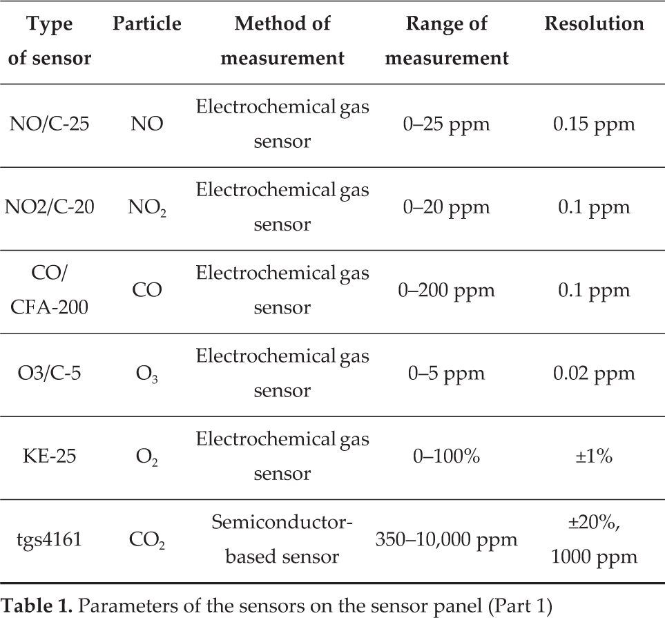
An intelligent measurement module that contains the detectors for air pollutants among other aerial particles and radiations: This should contain a microcontroller that pre-processes the measured data and stores them in a solid-state disc. This unit is connected to a radio modem, which is responsible for the real-time transfer of collected data. The AGL altitude (calculated from barometric pressure), speed over ground and position (provided by the global positioning unit) are directly transferred from the flight controller unit to the measurement module. These data are then merged with the measurement values detected by the sensors using a method described fully in Chapter 3. Currently, the module can measure the following air pollutants and components:

Oxygen (O₂)

Ozone (O₃)

Carbon dioxide (CO₂)

Carbon monoxide (CO)

Nitrogen dioxide (NO₂)

Nitrogen monoxide (NO)

Temperature

Humidity

PM10 particle count

Gamma radiation

UVA radiation

UVB radiation

The measurement module is capable of handling an additional 10 sensors. By replacing the gas detector modules, the detection of other particles could be performed as well. This high level of freedom guarantees a wide range of possible uses for the device.

The ground control software, responsible for the flight plan creation and management: This module should also check and verify the flight parameters during the flight. The ground station can be an arbitrary personal computer but, due to the typical environment of usage, it is more feasible to use a portable computer (laptop, notebook, or tablet) or a smart phone (currently Android or iOS) device. For practical application, it is advised that the computer should have an offline map database; there is usually no internet connection available at the location of the flight, so online map providers like Google or Bing maps cannot be used.

A ground modem with directional high-gain antenna that is directly connected to the ground control station: This unit is responsible for the real-time wireless communication between the aerial and ground units.

Data analysis and visualization software that can process and display the data received from the aerial unit: This module informs the user about the concentration and spatial distribution of air pollutants. Data can be displayed using either a traditional 2D or an advanced 3D interface. The advantage of the 2D interface is that it provides quantitative data that are easy to interpret according to the expectations of an engineer. The advantage of the 3D model is that it can provide a more general view; in this way, it is more suited to human thought mechanisms and thus helps facilitate the decision-making process.

The multi-rotor carrier is equipped with the measurement module in such a way that the sensors of the module can measure pollution directly, without any mechanical obstacles or barriers. The measurement module is placed below the plane of the rotors, so that the high-intensity airflow increases the amount of air that flows through the detectors. The electronics of the measurement module are connected directly to the flight controller. The module receives the air pressure, air and ground speed, GPS data and inertial measurements. The flight controller is also responsible for autonomous flight; this allows the device to be launched from a safe distance, in order to perform measurements in areas that could be hazardous or dangerous to humans.

2. Practical Implementation of a Measurement

Using the device, it is possible to perform a complex spatial examination of an area in a quick and efficient manner. Near to the supposed contaminated area, an ad-hoc ground station should be established that consists of the previously described parts. Using the ground control software, a flight path should be planned and the following aspects taken into consideration during the planning process:

From the launch point to the bounds of the measurement area, the flight speed should be optimal for the aerial vehicle (travel speed).

In the measurement area, the path should cover the pollution measurement area uniformly.

The flight speed over the polluted area must be set to match the reaction time of the sensors. This speed is characteristically a lot smaller than the approach speed.

After making a sweep of the area, the device should return to the launch point, once again travelling at the most optimal speed for the aerial vehicle.

For safety purposes, the total time of the flight must be lower than the maximum flight time permitted for the device.

If the given area cannot be fully covered in one flight, the measurement must be completed using multiple flights. When conducting multiple measurements this way, the order of the individual flights must be kept the same during the mission and the analysis.

3. Theoretical Processing of the Measurements

For the processing of the measurement data, we assume that during each flight (around 15 minutes) there is no significant change in the spatial distribution of the pollutants. We also assume that changes in the spatial distribution of the pollutants over time can be modelled using repeated measurements after a given unit of time (30 minutes, 60 minutes, etc.).

During the flight, the on-board device uses the available values to create a dataset with the following structure (1):

\begin{array}{l} {3 D c o o r d i n a t e s (x, y, z), \\ t i m e s t a m p, m e a s u r e m e n t d a t a (1 \dots n)} \end{array}

(1)

When processing the data, a timestamp can be used to separate the individual flights (the repeated measurements); thus, the first measurement is numbered as No. 1, the second as No. 2, and the Mth measurement as No. M. After this conversion, the following dataset is created (2):

\begin{array}{l} {3 D c o o r d i n a t e s (x, y, z), \\ I D o f m e a s u r e m e n t (1 \dots m), m e a s u r e m e n t d a t a (1 \dots n)} \end{array}

(2)

By displaying the series from 1 to M, we can show the changes in the spread of the pollutants over time.

4. Aspects of Planning the Flight Profile

The measurements can only be performed with accurate results if the appropriate retention time (t_s) has been used for the sensor. Typically electrochemical sensors have high retention time values; however, their size and mass are comparatively small, so they are ideal for small aerial vehicles. If there is not enough time to accommodate the full retention period, there are various extrapolation techniques to deduce the actual concentration of the pollutant. The principle is as follows:

The characteristic settling curve of the current sensor is known (the relationship between the current waiting time and the measured value), which is usually a non-linear correlation. Unfortunately, this correlation also depends on the measured concentration; however, for practical applications, the manufacturers usually provide one characteristic curve that describes the sensor reasonably well.

Figure 1.

The characteristic settling curve of the O₂ sensor

The characteristic curve of the oxygen sensor that is being used in the experimental device is a good example for all the applied sensors, since the curve can be closely approximated using (3):

f (x) = \frac{x_{2}}{1 + x_{1} e^{- x}} + c

(3)

where

x₂: 0.9552;

x₁: 3249; and

c: 0.008519.

The retention time of this sensor is 14 sec. Tables 3 –8 demonstrate the minimum diameter of the area required to measure the O₂ concentration, supposing that the concentration is constant within this area and the speed of the aerial vehicle is also known.

Table 1.

Parameters of the sensors on the sensor panel (Part 1)

Type of sensor	Particle	Method of measurement	Range of measurement	Resolution
NO/C-25	NO	Electrochemical gas sensor	0–25 ppm	0.15 ppm
NO2/C-20	NO₂	Electrochemical gas sensor	0–20 ppm	0.1 ppm
CO/CFA-200	CO	Electrochemical gas sensor	0–200 ppm	0.1 ppm
O3/C-5	O₃	Electrochemical gas sensor	0–5 ppm	0.02 ppm
KE-25	O₂	Electrochemical gas sensor	0–100%	±1%
tgs4161	CO₂	Semiconductor-based sensor	350–10,000 ppm	±20%, 1000 ppm

Table 2.

Parameters of the sensors on the sensor panel (Part 2)

Type of sensor	Retention time	Range of operation
NO/C-25	T90:<25sec	−20–45°C RH:15–90% 90–110KPa
NO2/C-20	T90:<60sec	−20–45°C RH:15–90% 90–110KPa
CO/CFA-200	T90:<40sec	−20–40°C RH:15–90% 90–110KPa
O3/C-5	T80:<60sec	−20–45°C RH:15–90% 90–110KPa
KE-25	T90:<14sec	5–40°C RH:10–90% 80–120KPa
tgs4161	T90:<1.5min	−10–50°C RH:5–95%

Table 3.

The required length of flight and retention times of some typical sensors at various carrier speeds (Part 1)

	Retention time of the NO sensor [sec]
	25	17.5
Speed [m/s]	Length of flight [m] 100%	Length of flight [m] 70%
20	500	350
10	250	175
5	125	87,5
2	50	35
1	25	17.5
0.5	12.5	8.75

Table 4.

The required length of flight and retention times of some typical sensors at various carrier speeds (Part 2)

	Retention time of the NO₂ sensor [sec]
	60	42
Speed [m/s]	Length of flight [m] 100%	Length of flight [m] 70%
20	1200	840
10	600	420
5	300	210
2	120	84
1	60	42
0.5	30	21

Table 5.

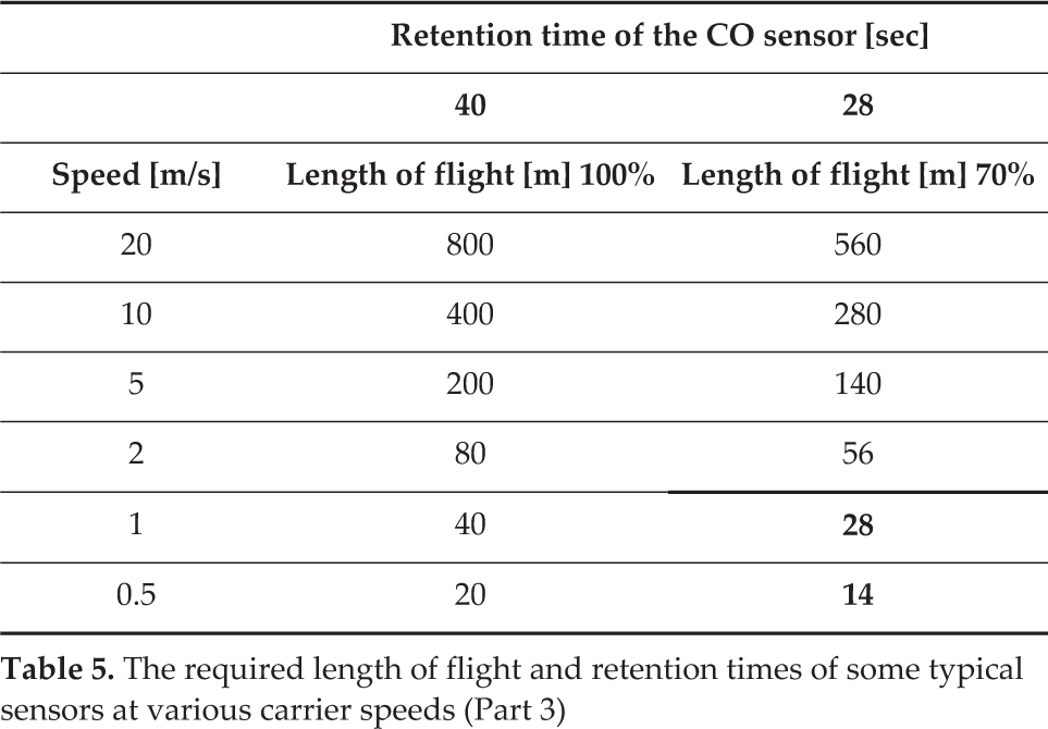
The required length of flight and retention times of some typical sensors at various carrier speeds (Part 3)

	Retention time of the CO sensor [sec]
	40	28
Speed [m/s]	Length of flight [m] 100%	Length of flight [m] 70%
20	800	560
10	400	280
5	200	140
2	80	56
1	40	28
0.5	20	14

Table 6.

The required length of flight and retention times of some typical sensors at various carrier speeds (Part 4)

	Retention time of the O₃ sensor [sec]
	60	42
Speed [m/s]	Length of flight [m] 100%	Length of flight [m] 70%
20	500	350
10	250	175
5	125	87.5
2	50	35
1	25	17.5
0.5	12.5	8.75

Table 7.

The required length of flight and retention times of some typical sensors at various carrier speeds (Part 5)

	Retention time of the O₂ sensor [sec]
	14	9.8
Speed [m/s]	Length of flight [m] 100%	Length of flight [m] 70%
20	1200	840
10	600	420
5	300	210
2	120	84
1	60	42
0.5	30	21

Table 8.

The required length of flight and retention times of some typical sensors at various carrier speeds (Part 6)

	Retention time of the CO₂ sensor [sec]
	90	63
Speed [m/s]	Length of flight [m] 100%	Length of flight [m] 70%
20	800	560
10	400	280
5	200	140
2	80	56
1	40	28
0.5	20	14

The precision of pollution detection and measurement can be increased using slower vehicle speeds.

By knowing the characteristic curve of a sensor, the real concentration of a pollutant can be estimated, even if the measurement time is shorter than the desired retention time. In this case, the actual concentration y_pollutant can be estimated using (4):

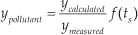
y_{p o l l u t a n t} = \frac{y_{c a l c u l a t e d}}{y_{m e a s u r e d}} f (t_{s})

(4)

where

y_calculated: the measured concentration returned by the sensor during a waiting time of 0.7t_s, so y_calculated = f(0.7t_s);

y_measured: actual measured concentration; and f(x): the function that approximates the characteristic curve of the sensor.

When there are large differences between the retention time and the actual waiting time, the uncertainty of the measurement can yield a reasonably large deviation in the estimated concentration. Sufficient accuracy can only be reached if the actual waiting time is positioned where the rise of the characteristic settling curve is slowing down. This is generally around 70% of the required retention time. In accordance with this, the flight speed must be determined so that the flying device spends at least 70% of the required retention time in the range of the minimally expected localization accuracy, which is 6 metres with an average GPS unit [4, 16, 17, 18, 20].

For example, if the NO concentration has to be determined with a localization accuracy of ±3 metres, using an NO sensor with a retention time of 25 seconds, then the aerial vehicle must make the 6-metre distance within 17.5 seconds. This is approximately 0.34 m/sec.

Figure 2.

Constant speed flight path using slow-settling sensors

The position of the pollution value measured by the sensor for each measurement point can be calculated using the measurement time and settling time (5):

P o s_{M e s u r e m e n t} = P o s_{A c t u a l} - P o s_{0.35 t_{s}}

(5)

When using even slower sensors, the flight path is best defined with predefined waiting points and fast transitions between them. The waiting points are equally spaced. This way, discrete measurement points can be evaluated and displayed in the same manner as above. In this case, measurement correction is not needed.

Figure 3.

Waiting-time-type flight path using extremely slow-settling sensors

5. Displaying the Obtained Data

The system is capable of displaying the measured data in real time using a 2D interface. This display mode makes it possible to modify the flight plan according to the spread of the pollutant particles. Since, in most cases, the pollution is not visible, the path of the initial flight can only be planned based on assumptions and personal experiences.

The real-time display provides the user with the feedback required to decide if the pollution is indeed inside the flight area or not. It is also possible that the pollutant is detected somewhere within the flight area, but that the concentration continuously increases towards one edge of the area. In this case, the path of the next measurement should be modified so it covers the whole polluted area. If this area is bigger than the largest area that can be observed in one flight, it can instead be measured using multiple flights.

The appearance of the 2D display mode is basically a function displayed in a Cartesian coordinate system. The two axes represent the geographical coordinate pairs; the measurements are taken in locations marked by these pairs. The concentration of the pollutant in a given location is marked by a coloured circle (disc), the radius “r” of which is proportional to the concentration of the pollutant. A single series of measurements represents the concentration values for the same altitude level, so the aforementioned diagram is created (layered) an additional time for each of the different altitude levels being measured during the flights. Within the various layers, the circles representing the pollutants form a “cloud” that can effectively be used to illustrate the polluted area at that specific altitude level.

The changes in the spread of pollutants over time can be clearly demonstrated by using an animation to display the consecutive individual measurements performed under the same conditions (on the same area, at the same altitude level). This information can also be used to give reasonably accurate estimations about the short-term changes in the size of the threatened area and about the severity of the situation.

The 3D interface is an extension of the 2D interface. In this case, the third axis of the coordinate system represents the altitude. Thus, the 3D display mode is similar to the 2D display mode, but with one change; to show the scale of the pollution, instead of circles we now use coloured spheres, with their radius “r” proportional to the measured concentration. Using the 3D display mode, it is now possible to use only one diagram instead of displaying multiple diagrams to represent multiple layers.

There are some enhancements that can be used with these display interfaces. For example, we could get rid of the circles or spheres with their radius “r” proportional to the measured concentration if we take into consideration the different models of gas dynamics [19, 21, 22]. By using these models, we can change the opacity levels of the circles and the spheres; alternatively, by using various approximation and interpolation techniques, we can create even more realistic “clouds”. The 3D cloud-generating method is ahead used on several area of sciences and engineering [23, 24, 25]. Advantages of the 3D technique include good comprehensibility and the fact that it is more immediately informative to the viewer. Although these techniques have a lot higher computational requirements (which could mean that the real-time display of the measurements might become impossible), they can still prove useful in many scenarios. Disaster prevention and damage control rescue specialists (who are not usually experts in the fields of gas dynamics and gas diffusion) could use these advanced display modes to make better subjective judgements. Such a technique for visualizing invisible pollutants (which essentially involve making the pollutant visible) could then be combined with their years of experience, and this would ensure that the decisions made and further actions taken would be more appropriate and more efficient.

6. A Possible Field of Use

The presented, patent-pending system could be efficiently used in cases of the unexpected emission of dangerous aerial pollution particles, or other environmental pollution involving dangerous gases or other hazardous vapours, that can affect a small area.

Since the weight of the measurement device and the ground station is reasonably small, the system is highly mobile. Therefore, it would be possible to transport the system quickly to the vicinity of the unexpected event and start taking measurements right away. During the measurements, the current pollution level can be immediately shown, and by using consecutive flights the spread rate of the pollution can be established as well. In addition, with sequential measurements, it is possible to indicate the activity of the pollutant particle source. If the concentration levels were seen to be rising, it would then be possible to make deductions about the increasing activity of the source, while it would be possible to estimate the depletion of the source or the success of any attempted solution if the concentration were seen to be decreasing.

By using multiple sensors simultaneously, it is possible to point out complex pollution patterns or multiple pollutant sources in one area. In this way, it is also possible to detect primary and secondary sources simultaneously (e.g., the direct leakage of hazardous material and its various reactions with components of the soil).

7. Advantages over Other Similar Devices

There are a number of other carrier devices that could be used to measure the concentration of various pollutants in the air.

By connecting the sensors to appliances that are lighter than air (balloons), the movements of the system would be reasonably low. This is good for slow-settling sensors; however, the usage of the balloons is heavily restricted due to weather conditions. The most common scenario for balloons is that they carry the sensors during their constant ascent until the balloon is destroyed at high altitudes, due to the expanding gas. This measurement method is usually used in the field of meteorology and the measured data can primarily be interpreted in relationship to altitude. However, this method is not capable of reiterated measurements of a small area at constant altitudes. There have been experiments in which a balloon is created so that it will only rise to a defined altitude; at this point, it will not perish, but instead drift according to the dominant wind at that altitude. In this case, the measurements are taken at the altitude of the drifting. Even though, in this case, it is possible to interpret the data in relationship to the geographical coordinate, this method is still not capable of the precise examination of small areas, because the altitude at which the drifting occurs cannot be exactly defined beforehand. Therefore, layered measurements are also not possible with this method.

Similarly, controlled lighter-than-air devices (airships) cannot normally be used in the practical environment, as they are too sensitive to the wind. Other disadvantages of these devices are that they are usually too large and the gas required to fill them up is expensive.

When using sensors fitted onto fixed-wing flying devices, it is possible to cover a reasonably large area, but the minimum possible speed of these devices is usually too high and, because of this (and due to the slow sensors), the accuracy of the measurements cannot be good enough to locate the emission source precisely, within less than a couple of square kilometres. There have, however, been a couple of meteorological experiments involving unmanned aerial vehicles (UAVs) [7, 8, 9]. The advantage of these UAVs is that it is possible to perform the measurements along previously defined spatial coordinates. Using our visualization method, this carrier is also capable (to a limited extent) of performing measurements to monitor the pollution levels and the changes in pollution within a given area; however, there are two main drawbacks of using a fixed-wing aeroplane. The first one is that the required measurement time of some of the sensors is very high compared to the flying speed of the plane. The retention time is around 20–30 seconds for several sensors, and during this time span, even a reasonably slow aeroplane flying at a moderate speed of 14 m/s will have flown around 280–420 metres. Because of this, we have to use reasonably fast sensors and relatively slow aeroplanes. Another disadvantage is that, with aeroplanes, it is not possible to perform safe and secure flights that are close to the ground. Because of this, these devices can usually be used only for measurements for which the minimal altitude is typically around 100 metres or more (this value is highly dependent on the aeroplane that is being used).

With sensors placed on helicopters, the covered area can be reasonably large and the speed of the flying devices can be arbitrarily slow (they can even hover above a given point). The disadvantage of these is the mechanical complexity of the system, which is reflected in both the price and the reliability of the helicopters. It is fairly complicated to set up these devices initially, and the constant replacement of deteriorated parts necessitates the frequent resetting or replacement of parts, along with additional initial set-ups.

By placing the sensors on multi-rotor devices, we can create a system that is reasonably slow (which is favourable for the slow sensors), but the device will also be capable of quick motion if required. The multi-rotor flying devices are less sensitive to the weather than balloons and they can be a lot more easily manoeuvred as well. Compared to helicopters, their mechanical layout is a lot simpler, so their reliability, operation and maintenance requirements are all a lot more favourable. Due to their simpler structure, it is also easier to set up the multi-rotor devices and not necessary to reset the parts frequently due to their deterioration. The electronic motors ensure the accuracy of the measurements as well, since the emission of the measurement system during its operation is zero.

As a conclusion, there are two devices that are suitable for the preliminary conditions. These are the traditional helicopter and the multi-rotor aerial vehicles. However, due to the additional advantages of the multi-rotor layout over traditional helicopters, the multi-rotor devices are better suited to the practical implementation of the measurements.

Figure 4.

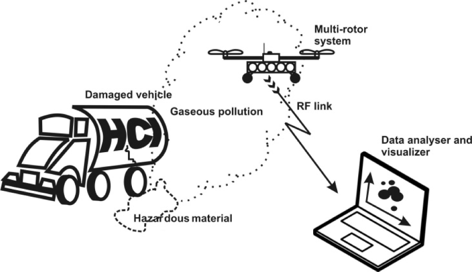
Application of the developed system

Figure 5.

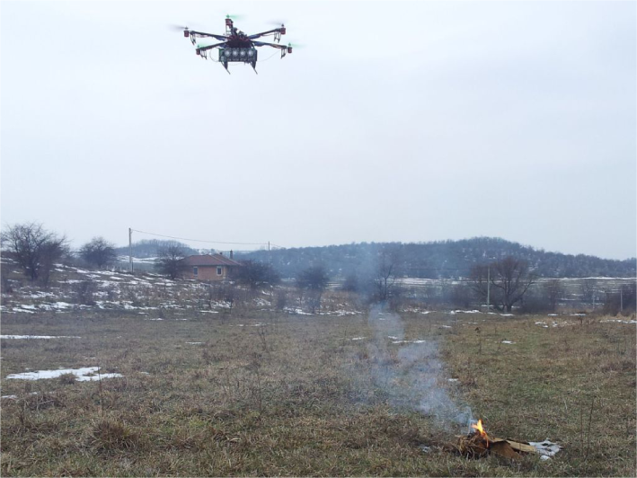
Experimental measurement

Figure 6.

2D visualization of the experimental CO automatic measurement

Figure 7.

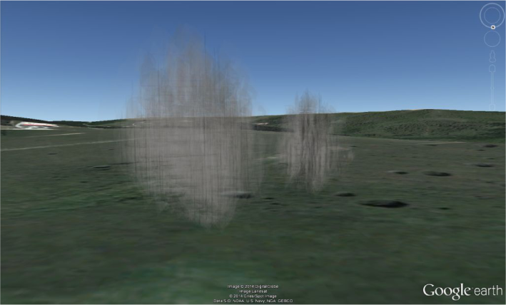
3D visualization of the experimental CO measurement

Figure 8.

2D visualization of the experimental NO₂ manual measurement

Figure 9.

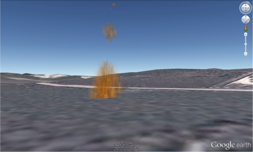
3D visualization of the experimental NO₂ measurement

References

Šmídl

Hofman

: “Tracking of atmospheric release of pollution using unmanned aerial vehicles”, Atmospheric Environment, Vol. 67, pp. 425–436, 2013.

Berman

E. S. F.

Fladeland

Liem

Kolyer

Gupta

: “Greenhouse gas analyzer for measurements of carbon dioxide, methane, and water vapor aboard an unmanned aerial vehicle”, Sensors and Actuators B: Chemical, Vol. 169, No. 1, pp. 128–135, 2012. Available from: http://www.elsevier.com/locate/snb

Khan

Schaefer

Tao

Miller

D.J.

Sun

Zondlo

M. A.

Harrison

W. A.

Roscoe

Lary

D. J.

: “Low Power Greenhouse Gas Sensors for Unmanned Aerial Vehicles”, Remote Sensing Vol. 4, No. 5, pp. 1355–1368, 2012. Available from: http://www.mdpi.com/journal/remotesensing

Morrison

Busch

: “Global Positioning Systems (GPS) accuracy report”, Wisconsin Department of Natural Resources, Madison, WI, 2001. Available from: http://dnr.wi.gov/maps/gis/documents/gps_accuracy.pdf

Zhao

Ochieng

W. Y.

Quddus

M. A.

Noland

R. B.

: “An Extended Kalman Filter algorithm for Integrating GPS and low-cost Dead reckoning system data for vehicle performance and emissions monitoring”, Journal of Navigation, Vol. 56, pp. 257–275, 2003.

Hunt

E. R.

Daughtry

C. S. T.

Walthall

C. L.

McMurtrey

J. E.

Dulaney

W. P.

, “Agricultural remote sensing using radio-controlled model aircraft”, in: Van Toai

Major

McDonald

Schepers

Tapley

(eds.), Digital Imaging and Spectral Techniques: Applications to Precision Agriculture and Crop Physiology, ASA-CSSA-SSSA, Madison, WI, pp. 197–205, 2003.

Holland

G. J.

Webster

P. J.

Curry

Tyrell

Gauntlett

Brett

: “The Aerosonde Robotic Aircraft: A New Paradigm for Environmental Observations”, Bulletin of the American Meteorological Society, Vol. 82, No. 5, pp. 889–901, 2001.

McGeer

: “LAIMA: The first Atlantic crossing by unmanned aircraft”, The Insitu Group, Bingen WA, 1999. [electronic paper]

Curry

Maslanik

J. A.

Holland

Pinto

J. O.

: “Applications of Aerosondes in the Arctic”, Bulletin of the American Meteorological Society, Vol. 85, No. 12, pp. 1855–1861, 2004.

10.

Adams

D.A.

Fry

Gurk

Hudgens

Newell

Singleton

Smith

C. R.

: “Advanced study of coastal zone oceanographic requirements for ERTS E and F”, National Technical Information Service, N71-28328, 1971.

11.

Acevedo

J. J.

Arrue

B. C.

Diaz-Banez

J. M.

Ventura

Maza

Ollero

: “Decentralized strategy to ensure information propagation in area monitoring missions with a team of UAVs under limited communications”, Unmanned Aircraft Systems (ICUAS), 2013 International Conference on, pp. 565–574, 2013. Available from: http://dx.doi.org/10.1109/ICUAS.2013.6564734

12.

Kingston

Beard

R. W.

Holt

: “Decentralized perimeter surveillance using a team of UAVs”, Robotics, IEEE Transactions on, Vol. 24, No. 6, pp. 1394–1404, 2008.

13.

Smith

S. L.

Rus

, “Multi-robot monitoring in dynamic environments with guaranteed currency of observations”, in Decision and Control (CDC), 2010 49th IEEE Conference on, pp. 514–521, 2010.

14.

Maza

Caballero

Capitan

Martinez-de-Dios

J. R.

Ollero

, “A distributed architecture for a robotic platform with aerial sensor transportation and self-deployment capabilities”, Journal of Field Robotics, Vol. 28, No. 3, pp. 303–328, 2011.

15.

Viguria

Maza

Ollero

, “Distributed service-based cooperation in aerial/ground robot teams applied to fire detection and extinguishing missions”, Advanced Robotics, Vol. 24, No. 1–2, pp. 1–23, 2010.

16.

Laliberte

A. S.

Rango

Herrick

J. E.

: “Unmanned Aerial Vehicles for rangeland mapping and monitoring: A comparison of two systems”, Proceedings of the American Society for Photogrammetry and Remote Sensing Annual Conference, Tampa, FL, 2007.

17.

Serr

Windholz

Weber

: “Comparing GPS receivers: A field study”, Journal of the Urban and Regional Information Systems Association, Vol. 18, No. 2, pp. 19–24, 2006.

18.

Gehring

Lander

: “GPS Lens - GPS based controlling of pointers on large-scale urban displays using mobile devices”, Proceedings of the International Symposium on Pervasive Displays, Mountain View, CA, 2013.

19.

Combi

M. R.

Harris

W. M.

Smyth

W. H.

: “Gas Dynamics and Kinetics in the Cometary Coma: Theory and Observations”, in: Festou

M. C.

Keller

H. U.

Weaver

H. A.

(eds.), Comets II, University of Arizona Press, Tucson, AZ, pp. 523–552, 2004.

20.

Hedgecock

Maroti

Sallai

Volgyesi

Ledeczi

: “High-accuracy differential tracking of low-cost GPS receivers”, Proceeding of the 11th Annual International Conference on Mobile Systems, Applications, and Services, pp. 221–234, 2013.

21.

Khelil

Naji

Loukarfi

Mompean

: “Prediction of a high swirled natural gas diffusion flame using a PDF model”, Fuel, Vol. 88, No. 2, pp. 374–381, 2009. Available from: http://dx.doi.org/10.1016/j.fuel.2008.09.008

22.

Ilbas

Yilmaz

Kaplan

: “Investigations of hydrogen-hydrocarbon composite fuel combustion and NO_x emission characteristics in a model combustor”, International Journal of Hydrogen Energy, Vol. 30, No. 10, pp. 1139–1147, 2005.

23.

Lafarge

Mallet

: “Creating large-scale city models from 3D-point clouds: a robust approach with hybrid representation”, International Journal of Computer Vision, Vol. 99, No. 1, pp. 69–85, 2012.

24.

Fielding

M. D.

Chiu

J. C.

Hogan

R. J.

Feingold

: “3D cloud reconstructions: Evaluation of scanning radar scan strategy with a view to surface short-wave radiation closure”, Journal of Geophysical Research: Atmospheres, Vol. 118, pp. 1–15, 2013.

25.

Vosselman

Dijkman

: “3D Building Model Reconstruction from Point Clouds and Ground Plans”, International Archives of Photogrammetry and Remote Sensing, Vol. XXXIV-3/W4, pp. 37–43, 2001.

A Multi-Rotor System for the Collection and Analysis of Measurements to Evaluate and Spatially Demonstrate the Pollutants in the Air

Abstract

Keywords

1. Introduction

2. Practical Implementation of a Measurement

3. Theoretical Processing of the Measurements

4. Aspects of Planning the Flight Profile

5. Displaying the Obtained Data

6. A Possible Field of Use

7. Advantages over Other Similar Devices

References