Designation and Control of Landing Points for Competitive Robotic Table Tennis

Abstract

Competitive robotic table tennis involves many topics such as smart ball returning strategy, precise motion control, etc. It remains a quite challenging task due to the unpredictable, uncooperative incoming ball and the requirement of a smart strategy to defeat the opponent. Designation and control of landing points is one basic aspect of ball returning strategies in competitive robotic table tennis because different landing points require the opponent to make different efforts to return the ball. In this paper, we present a method to designate desired landing points based on competitiveness level. We also propose a learning based landing point control approach to minimize the error of the actual landing points with respect to the designated landing points. The proposed methods have been verified through experiments on a humanoid table tennis robot.

1. Introduction

Robotic table tennis is an excellent but challenging task. It involves many research topics such as visual servo, trajectory generation, ball returning strategy, etc. Robot table tennis can be divided into cooperative table tennis and competitive table tennis. Cooperative table tennis means that the ball is returned in a way such that the ball will be suitable for the opponent to hit. Here the word “suitable” means a robot player could return a ball without large changes of the joint angles. On the other hand, competitive table tennis targets at returning the ball in a way such that the ball will be unsuitable for the opponent to hit, which makes the opponent fail in the competition. Although cooperative playing is not difficult any more, competitive robotic table tennis remains quite challenging because most of the incoming ball is much faster and much further, and ball returning is more strategic and challenging. This paper addresses the landing point designation and control problems for competitive robotic table tennis.

Robot table tennis has attracted much attention since the early studies ([1, 2, 3]). Some studies have made many explorations on hardware design. Other studies have paid much attention to robust vision perception algorithms and generation of anthropomorphic ball hitting motions. During the last decades, the persistent interests in robotic table tennis studies still attracted researchers from all over the world. Acosta et al. [4] constructed a PC based low-cost ping-pong robot. Using an improved version of a learning method in paper [5], Miyazaki et al. [6, 7] presented a kind of robotic learning approach for robot table tennis. Studies on visual perception and prediction of table tennis balls were presented in [8,9,10]. Mulling and her group focused on anthropomorphic striking movement generation for a table tennis robot [11,12]. As far as humanoid table tennis robot is concerned, the balance maintenance was discussed in paper [13]. We have also developed a humanoid robot which is able to rally with human players or another robot player, and the best record of cooperative playing (robot vs robot) is more than 200 rounds [14,15,16,17,18,19,8]. Most of the proposed robots were designed for cooperative table tennis playing, and have achieved a great success. However, competitive robotic table tennis is not deeply investigated yet.

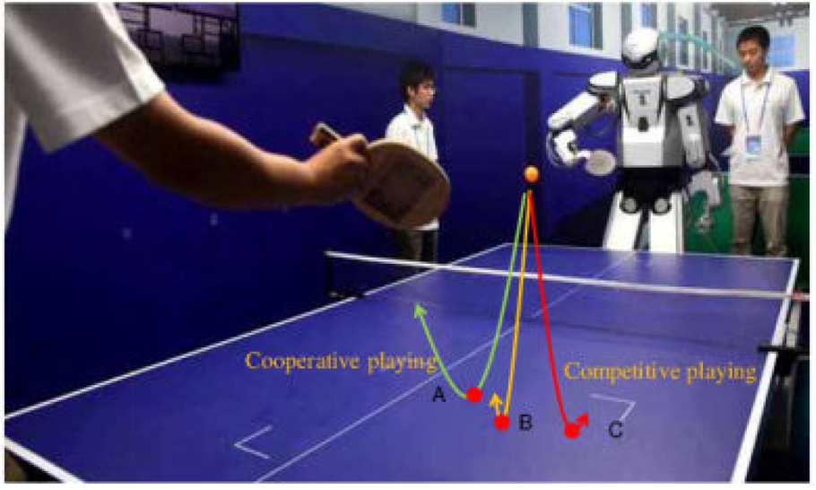
A landing point is the position where the returned ball lands on the opponent's table. It is important for competitive robotic table tennis. Since different landing points usually require the opponent players to make quite different efforts, choosing a specific landing point in each round is one of the most effective strategies to win the game. As shown in Figure 1, it will be more and more competitive when the landing point moves from A → B and B → C. A is most suitable for cooperative ball returning, while C is most suitable for competitive ball returning. Once we have designated a landing point, we should control the emergent velocity of the ball so as to return the ball to the desired landing point. Although designation and control of landing points is such a basic and important issue in competitive robotic table tennis, to our knowledge, however, only a tiny amount of the previous studies have addressed the problem. Paper [4] designed an expert control or game strategy planning approach for landing point determination of a ping-pong player prototype. However, this study did not discuss how to improve the accuracy of landing point control. Huang et al. [20] proposed an effective controller based on active and lazy learning for a ping-pong playing robot to return the incoming ball to a desired position. A recent study [21], from a biological viewpoint, modelled human strategies in table tennis playing using inverse reinforcement learning and provided discussions on some relevant features, such as landing point of the ball and velocity of the ball which are not ignorable in ball returning. In order to explore the basic issues of competitive robotic table tennis, a method to designate landing points for ball returning, and a learning control method to reduce errors between the actual and desired landing points will be presented in this paper. We will prove that our approach is effective for competitive robot table tennis.

Figure 1.

Different landing points during robotic table tennis playing

The rest of the paper is organized as follows. In Section 2, an optimized waiting posture is introduced to maximize the manipulability of a robot when it is waiting for an incoming ball. A landing point designation method for competitive ball returning is given in Section 3. Section 4 proposes the landing point error reduction control method to return the ball to the desired landing point. After the proposed methods are verified through experiments on a humanoid robot in Section 5, the paper is concluded finally in Section 6.

2. Waiting posture optimization

A waiting posture is an state of a robotic arm in the waiting stage [22, 23] when the robot is waiting for the opponent to return a ball back. The waiting posture should be optimized so that the robot could return a ball with shortest distance and least efforts in average. This section proposes a method to choose an optimal waiting posture using manipulability indexes and joint limits.

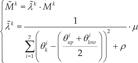
In the waiting stage, human or robot players usually place a racket with “comfortable” joint configurations so that the arm consumes only a little energy and is convenient to move the racket. Especially, this configuration is called a waiting posture of a robot. In order to maximize the quick response capability to the incoming ball, the manipulability index [24] can be used to optimize the waiting posture of a robot. Let ${\theta }_k^i(i=\mathrm{1,2,}\cdots \text{,7})$ be the k^th joint angle configuration of the 7-Dof (Degree of freedom) robotic arm of our humanoid robot, given the upper and lower limits of these joint angles, the k^th manipulability M^k with respect to the k^th joint configuration, can be calculated using $M^k=\sqrt{\det J^k{(J^k)}^T}$ , where J^k and (J^k) ^T are the Jacobian and the transpose of the Jacobian of the k^th joint configuration. The optimal waiting posture for the robot is determined by the configuration of joints which maximizes the manipulability M^k.

On the other hand, joint angle limits and collision avoidance constraints should also be taken into consideration. So the extended manipulability, or the manipulability penalized by the joint angle limits and collision conditions [25], is used instead. The extended manipulability $M_{ex}^k$ can be calculated by the augmented Jacobian ${\tilde{J}}^k=L^k\cdot O^k\cdot J^k$ , where L ^k and O^k are joint limit penalization matrix and collision penalization matrix of the k^th joint configuration.

In our application, the workspace is fairly free and so the collision constraints is ignored. For simplification, the manipulability can be updated as

$$\{\begin{array}{l}{\tilde{M}}^k={\tilde{\lambda }}^k\cdot M^k\hfill \\ {\tilde{\lambda }}^k=\frac{1}{{\displaystyle \sum _{i=1}^7}{\left({\theta }_k^i-\left(\frac{{\theta }_{up}^i+{\theta }_{low}^i}{2}\right)\right)}^2+\rho }\cdot \mu \hfill \end{array}$$

(1)

Where ${\tilde{M}}^k$ is the updated manipulability considering joint angle limits, ${\tilde{\lambda }}^k$ is the evaluating factor of the joint limits on manipulability, ${\theta }_k^i$ is the i^th joint angle of the k^th configuration, ${\theta }_{up}^i$ and ${\theta }_{low}^i$ are the i^th upper and lower joint angle limits, μ is an adjustable coefficient, and ρ >0 is an adjustable coefficient with small norm. When any joint angle is close to its limits, i.e. ${\theta }_{up}^i$ or ${\theta }_{low}^i$ , ${\tilde{M}}^k$ will be penalized.

Figure 2 illustrates the exemplified manipulability measurement of each arm configuration in the chosen workspace. The workspace is defined under the shoulder frame. An arm configuration is formed by the value of all the joint angles, ${\theta }^i(i=\mathrm{1,2,}\cdots \text{,7})$ . All the joint configurations of the robot have a common shoulder position with respect to the table tennis table. (The table's position, or the origin of frame O _w1 XYZ in Figure 5, is [−2.963m,-0.325m,-0.765m] ^T under the shoulder coordinate frame.) The upper and lower limits of each joint angle can be given to choose the workspace where the optimized waiting posture will be produced. The upper limits of the joint angles are (60°,-30°,100°,100°,100°,10°,45°). The lower limits of the joint angles are (30°,-60°,80°,60°,80°,-10°,25°). The step (interval) of the optimization procedure is set as 5° for each joint for simplification. By calculation, the optimized waiting posture without joint limits is at the arm configuration of (55°,-60°,100°,75°,80°,10°,25°). The optimized waiting posture with joint limits is at the arm configuration of (45° −60°,90°,80°,100°,-10°,35°).

Figure 2.

Manipulability with different joint configurations. For each end-effector position, the optimal manipulability index based on the joint configuration space is calculated.

3. Designation of Landing points

The ball returning strategy is the way the robot returns the ball to the opponent's court with the aim of defeating the opponent. The desired position where the ball will landing on the opponent's court, which is called a landing point, is one of the key factors of the ball returning strategy. Actually, the position of the landing point with respect to the opponent's racket has a great impact on the difficulty of returning the ball back. This section will focus on the evaluation of the competitiveness of an arbitrary landing point and the designation of landing points in each round with a given competitiveness level.

3.1 Competitiveness index: evaluation of the competitiveness level of a landing point

In order to evaluate the competitiveness of an arbitrary landing point, we presents competitiveness index based on the position of the landing point.

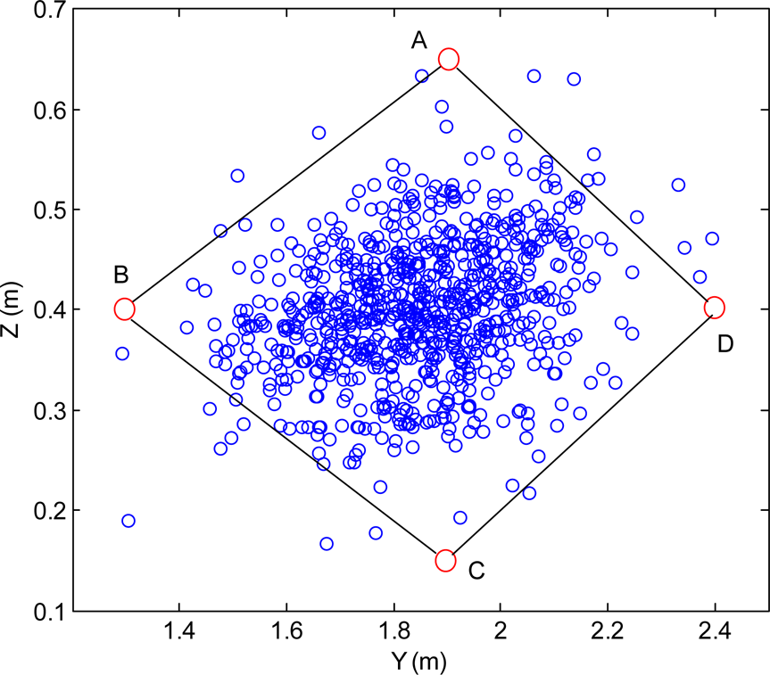
We use C_id as an index to describe the competitiveness of an incoming ball. A larger possibility for competitive playing of a designated landing point leads to a larger competitiveness index C_id. In order to obtain the competitiveness of an arbitrary landing point on the opponent's table, we introduce a polyhedron to illustrate our method in detail. In Figure 3, all the points are under the shoulder coordinate frame with O _s as its origin. The robot is in the waiting stage with elbow pose P _e and racket pose P ₁. In the figure, we have a polyhedron P _O ABCD . The polygon ABCD on the opponent's table represents the potential landing area which is obtained by experimental trials. A smallest polygon ABCD that contains most of the experimental samples will be chosen as the potential landing area. Inside the polygon ABCD , there is a landing point P _OO which is most suitable for the player to return the incoming ball. This landing point has the largest possibility for cooperative playing and the smallest possibility for competitive playing. If the ball lands outwards to the points in the boundary lines, e.g. the lines AB, BC, CD and DA of the polygon ABCD , the possibility for cooperative playing will decrease and the possibility for competitive playing will increase. The arbitrary point P _O of the polyhedron P _O ABCD is on the top of P _OO . We should point out that the height of the point P _O represents a highest cooperative level or a lowest competitive level. The points' height on the surface of the polyhedron (other than polygon ABCD ) relative with the height of P_O is meaningful. But the absolute height of these points, including P _O , has no meaning at all. For each point in the polygon ABCD, there will be a corresponding point, which has the same Y and Z coordinate value, on the surface of the polyhedron P _O ABCD . Actually, the corresponding point is the inverse projection of that point along X axis. The height of the corresponding point could be used to calculate the competitive level. We define f as the function that maps the points in the surfaces P _O AB, P _O BC, P _O CD , and P _O DA to their vertical projective points in the polygon ABCD along the X axis, and f⁻¹ as the inverse mapping. That is to say, f( P _O )→ P _OO , and f⁻¹( P _OO )→P_O. Then, we define the function x that denotes the x component of a point. A simple way to express C_id is

Figure 3.

Landing point planning of the returning ball

$$C_{id}=F\left(\chi \left(f^{-1}\left(P_{arb}\right)\right)\right)$$

(2)

Where P _arb is a potential landing point in the polygon ABCD, F is a bounded function. One possible form of F is

$$\{\begin{array}{l}F\left(x\right)=e^{-K(x)}\hfill \\ K\left(x\right)=\frac{x-\chi \left(A\right)}{\chi \left(P_O\right)-\chi \left(A\right)}\hfill \end{array}$$

(3)

Note that the arbitrary P _O is located above the table, which means that X( P _O )>X( A ).

Given any landing point in the polygon ABCD , the competitiveness index C_id can be obtained according to Equation (2) and (3). C_id will have a range of 1/e<C_id<1.

3.2 Landing point designation based on competitiveness index

Given an arbitrary landing point P , we can calculate its competitiveness level according to Equation (2). On the other hand, given a competitiveness value C, we should also designate a landing point P satisfying C_id = C.

However, there are many landing points sharing the same competitiveness value. Actually, the points whose inverse projective points have the same height on the surface of the polyhedron P _O ABCD excluding the polygon ABCD have the same competitiveness value. For example, In Figure 3, points aa, bb, cc, dd are in the polygon ABCD , points a, b, c and d are inverse projective points of aa, bb, cc and dd . Points in the lines ab, be, cd, da are inverse projection along X axis of the points in the lines aabb, bbcc, ccdd , and ddaa. a, b, c, d are points in the lines P _O A, P _O B, P _O C , and P _O D . ab, bc, cd , and da are lines in the surfaces P _O AB, P _O BC, P _O CD and P _O DA . The points in the polygon abcd have the same height, e.g., X(b). It is obvious that points in the lines of aabb, bbcc, ccdd, ddaa , produce the same competitiveness index F(X(b)) = C.

In order to remove ambiguity, we can choose a point in lines aabb, bbcc, ccdd , and ddaa that maximizes the distance to the point P _OO as the landing point corresponding to the competitiveness level C. So the procedures for designating the landing point with a given competitiveness index C are summarized as below.

Find the x value that produces the expected competitiveness index C using the Equation (2) and (3).

Find the original candidate points in the polyhedron P _O ABCD that share the same x value, e.g., we will obtain points in the lines ab, bc, cd , and da .

Calculate the candidate landing points by projection of the original candidate points using f function, e.g., we will obtain points in the lines aabb, bbcc, ccdd , and ddaa .

Choose the landing point that has the maximal distance to P _OO as the optimized landing point. If there are several landing points meeting this requirement, the landing point that has the maximal distance to the end-effector's waiting position is chosen as the optimized landing point. If there are still many landing points meeting the second requirement, randomly choose a point from them as the optimized landing point.

4. Learning based landing point control

Once we have got an optimized landing point according to the competitiveness index C, we should calculate the emergent velocity command of the returning ball. Due to the perception error, the motion error and the system error, the actual landing point is not the same as the desired landing point. This section presents a learning based landing point control method to adjust the velocity command of the returning ball so as to minimize the error between the desired landing point and the actual landing point.

4.1 The structure of the learning method

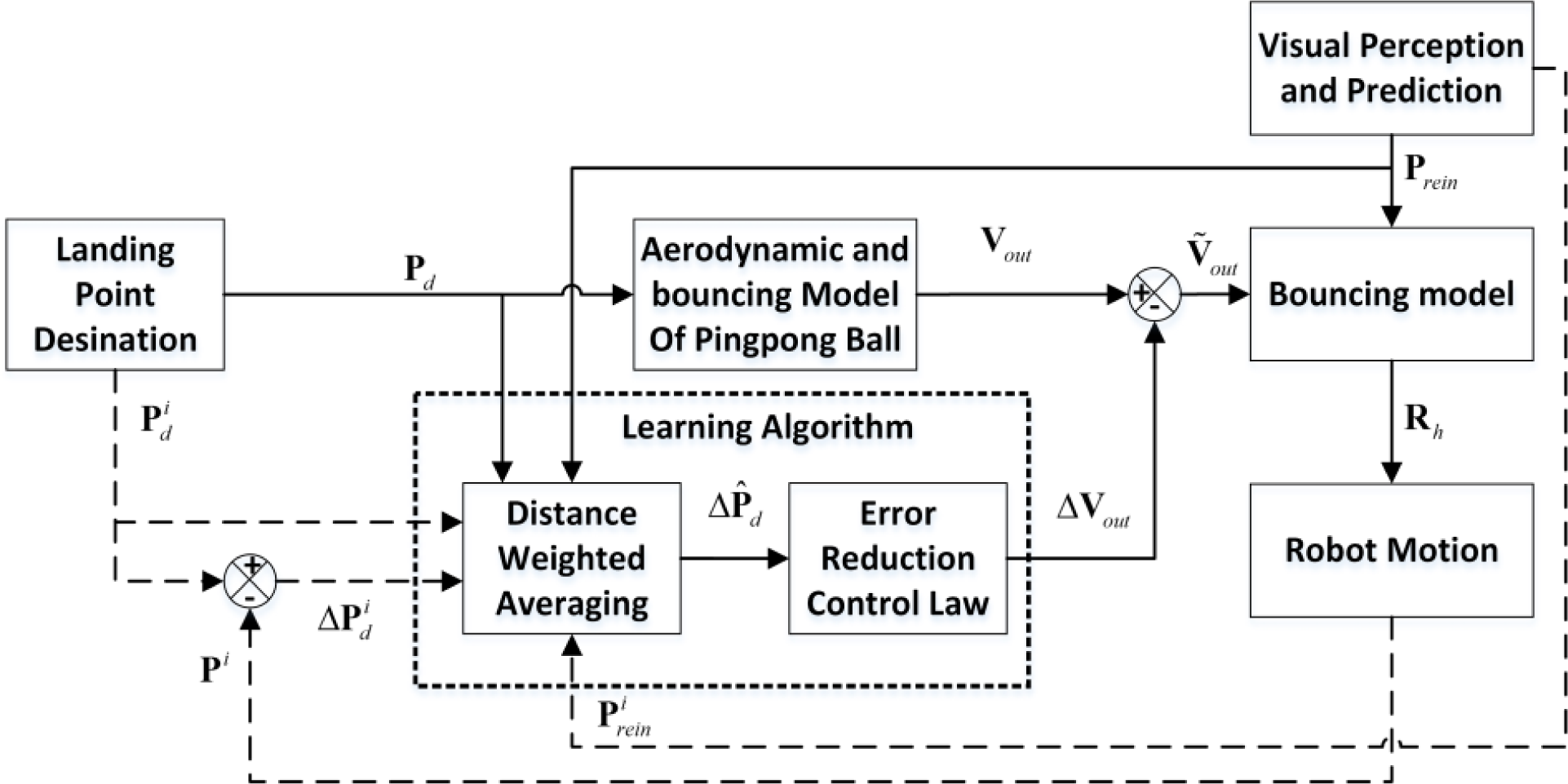
Figure 4 illustrates the structure of our learning based landing point control method. P_d = [0,P_dy,P_dz] ^T is the desired landing point. P is the actual landing point. Δ P _d is the landing error. $\mathrm{\Delta }{\widehat{P}}_d$ is the weighted landing error using Distance Weighted Averaging [26]. V _out =[V_outx,V_outy,V_outz] ^T is the desired velocity command of the returning ball just after ball-racket impact. Δ V _out =[ΔV_outx,ΔV_outy,ΔV_outz] ^T is the compensative delta velocity command of the returning ball obtained by the learning based landing point control method. ${\tilde{V}}_{out}=V_{out}+\mathrm{\Delta }{V}_{out}$ is the adjusted velocity command of the returning ball. P _rein =[P_inx,P_inz,V_inx,V_iny,V_inz] ^T is the predicted position and velocity of the incoming ball just before ball-racket impact. Here P_iny is neglected because it is always of the value y_h, which means that position and velocity of the incoming ball at the plane y = y_h is predicted. $R_h=[V_x,V_y,V_z,\alpha ,\beta ,\gamma {]}^T$ is the velocity and attitude of the racket when the incoming ball is returned. In the figure, the data with a top-right superscript i means that they are obtained off-line WITHOUT a learning method.

Figure 4.

Structure of the learning based landing point control method. The dashed arrows mean that the data with a top-right superscript i is the off-line data obtained WITHOUT a learning method. The solid arrows mean that the modules are running on-line WITH the learning method.

Given a desired landing point P _d , the returning velocity command V _out of the ball can be derived by the aerodynamic model and the bouncing model of the ball [8,12] or by the mapping method [6, 7]. However, due to the aerodynamic model [8] errors, the bouncing model [8] errors, robot motion errors and perception errors, the returning velocity command V _out itself is not enough to return the ball precisely without compensation. An overall system error should be compensated to improve the landing point control precision. In this paper, a delta velocity command of the returning ball Δ V _out , which is optimized by our learning based control method, is added to the returning velocity command V _out to minimize the error between the actual land points and the desired landing points. They are applied to obtain the compensative velocity command. Then, the desired racket motion R_h is derived based on the ball-racket bouncing model [8], the incident velocity V _in =[V_inx,V_iny,V_inz] ^T and the emergent velocity command ${\tilde{V}}_{out}$ . Finally, once R _h is known, motion planing and servoing of the robot arm could be carried out to return the incoming ball.

The learning method is composed of a Distance Weighted Averaging method [26] and an error reduction control law. In the off-line stage, The robot returns the ball without the learning method. The data with a top-right superscript is saved. In the on-line stage, the learning method uses the off-line data and current designated landing point command to estimate a potential landing error based on Distance Weighted Averaging, and then an error reduction control law is applied to generate the compensative the emergent velocity command Δ V _out . This command is added to the original V _out to reduce the landing point error.

4.2 Learning based landing point control

The learning method is to optimize the current compensative delta velocity Δ V _out to minimize the potential error between the designated landing point and the future landing point based on historic ball returning records.

1. Estimation of landing point errors

Considering that a desired landing point is variable in each ball returning round, the potential landing error (the error between the designated landing point and the future landing point in the current round) is estimated in advance, and a compensative delta velocity Δ V _out is optimized to reduce this potential landing error.

For simplification, the error estimation in the Y axis is analyzed in detail. Suppose that when the i^th incoming ball arrives at the predefined hitting plane y = y_h (y_h is constant, and the impact of the ball and racket occurs in the hitting plane), the detected position and velocity vector is $P_{rein}^i=[P_{inx}^i,P_{inz}^i,V_{inx}^i,V_{iny}^i,V_{inz}^i{]}^T$ . Under this condition, the desired landing point $P_{dy}^i$ will lead to error $\mathrm{\Delta }{P}_{dy}^i$ . We define ${[p_{re}^i{}^T,\mathrm{\Delta }{P}_{dy}^i]}^T$ as the i^th group of measured data, where $p_{re}^i=[P_{rein}^i{}^T,P_{dy}^i{]}^T$ . N groups of measured data (N should be greater than 100.) with many different landing points are collected and employed to estimate the error $\mathrm{\Delta }\widehat{P_{dy}}$ using Distance Weighted Averaging [27, 26, 28], if the information $q=[P_{rein}{}^T,P_{dy}{]}^T$ of the new incoming ball and the desired landing point is given. Here, Distance Weighted Averaging, the key elements of which were presented in paper [26], is not a new learning method, but it is first applied in the challenging competitive robotic table tennis.

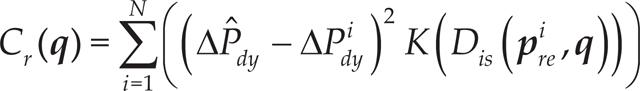
The cost function C_r( q ) weighting the discrepancy between the estimated error $\mathrm{\Delta }{\widehat{P}}_{dy}$ and the actual error $\mathrm{\Delta }{P}_{dy}^i$ resulted from each group of the measured historic data is expressed as

$$C_r(q)={\displaystyle \sum _{i=1}^N}\left({\left(\mathrm{\Delta }{\widehat{P}}_{dy}-\mathrm{\Delta }{P}_{dy}^i\right)}^{2}K\left(D_{is}\left(p_{re}^i,q\right)\right)\right)$$

(4)

Where K(·) is the weighting function and $D_{is}(p_{re}^i,q)$ is the Euclidean distance from q to $p_{re}^i$ . In fact, the estimation is obtained through memory-based learning method, and a high relevance is given to the nearby measured data.

The estimation of ΔP_dy should minimize the cost C_r( q ), and this estimation is derived by solving the function $\partial C_r/\partial \mathrm{\Delta }{\widehat{P}}_{dy}=0$ .

$$\mathrm{\Delta }{\widehat{P}}_{dy}\left(q\right)=\frac{{\displaystyle \sum }\mathrm{\Delta }{P}_{dy}^{i}K\left(D_{is}\left(p_{re}^i,q\right)\right)}{{\displaystyle \sum }K\left(D_{is}\left(p_{re}^i,q\right)\right)}$$

(5)

Since each component of q or $p_{re}^i$ may play a different role in determining the error, i.e., the detected positions and velocities of the incoming ball and the desired landing point contribute to error occurrence with varying degrees, a diagonally weighted Euclidean distance is chosen.

$$\begin{array}{l}{D}_{is}\left(p_{re}^i,q\right)=\sqrt{{\displaystyle \sum _j}{\left(n_j\left(p_{re}^{ij}-q^j\right)\right)}^2}\hfill \\ =\sqrt{{\left(p_{re}^i-q\right)}^T{N}^{T}N\left(p_{re}^i-q\right)}\hfill \end{array}$$

(6)

where n_j is the scaling factor for the j^th component and N is the diagonal matrix with N_jj=n_j.

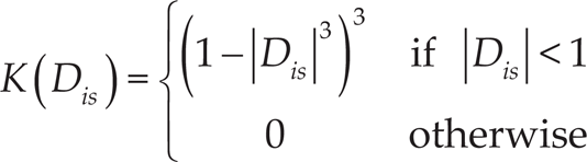
Although there are many different kernel functions available, we choose the Tricube kernel [28] (see (7)) because this kernel has a bounded extent, continuous first-order and second-order derivatives, which ensures continuous first-order and second-order derivatives of the estimation.

$$K\left(D_{is}\right)=(\begin{array}{cc}{\left(1-{\left|D_{is}\right|}^3\right)}^3& \mathrm{if}\left|D_{is}\right|<1\\ 0& \mathrm{otherwise}\end{array}$$

(7)

2. Error reduction control Law

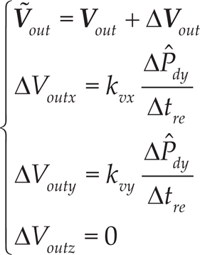
So, the landing error can be reduced by compensating the velocity command of the returning ball using the following equation

$$\{\begin{array}{l}{\tilde{V}}_{out}=V_{out}+\mathrm{\Delta }{V}_{out}\hfill \\ \mathrm{\Delta }{V}_{outx}=k_{vx}\frac{\mathrm{\Delta }{\widehat{P}}_{dy}}{\mathrm{\Delta }{t}_{re}}\hfill \\ \mathrm{\Delta }{V}_{outy}=k_{vy}\frac{\mathrm{\Delta }{\widehat{P}}_{dy}}{\mathrm{\Delta }{t}_{re}}\hfill \\ \mathrm{\Delta }{V}_{outz}=0\hfill \end{array}$$

(8)

Where ${\tilde{V}}_{out}$ is the compensated returning ball velocity command with error reduction method, k_vy and k_vx are adjustable coefficients, Δt_re is the time of the returning ball required to land on the table, and the time can be calculated in advance.

5. Experiments

In order to verify our proposed method for competitive table tennis playing, the humanoid robot BHR-5[15] is used as the table tennis robot. The humanoid table tennis system is illustrated in Figure 5, where P is the racket fixed on the robot (under the shoulder coordinate frame O _s XYZ ), CA and CB are cameras used to detect the trajectories of the ball from the opponent to the robot (under the coordinate frame O _w1 XYZ ) and CC and CD are cameras used to detect the trajectories of the ball returned by the robot (under the coordinate frame O _w2 XYZ ). All the cameras are connected to a PC, which communicates with the robot using CAN-Open and WIFI and produces P _rein and the actual landing point information for the robot.

Figure 5.

System of the robotic table tennis playing

To determine the potential region of the landing points, more than 1000 rounds of ball playing have been tried. The distribution of the landing points under O _w2 XYZ is shown in Figure 6. We will find a polygon ABCD that contains more than 97 percent of the experimental samples while keeping a maximal landing point density. The approximated boundary points for the region are A = [0m,1.9m,0.65m] ^T , B =[0m,1.3m,0.4m] ^T , C =[0m,1.9m,0.15m] ^T and D =[0m,2.4m,0.4m] ^T . In the table tennis playing experiments, the point [0m,1.9m,0.4m] ^T is found most suitable for the opponent player to hit the ball, and this point is set as P _OO . (The point P_OO may be different in real applications when the robot and the opponent stands in different places.) In the experiments, X( P _O ) is set as 0.6, and the landing point position can be derived once the competitiveness index is given. The competitiveness indexes are given as $C_{id}=e^{-\frac{0.4}{0.6}}$ , $C_{id}=e^{-\frac{0.35}{0.6}}$ , $C_{id}=e^{-\frac{0.3}{0.6}}$ and $C_{id}=e^{-\frac{0.25}{0.6}}$ , which correspond to the desired landing points of [0m,1.7m,0.4m] ^T , [0m,1.65m,0.4m] ^T , [0m,1.6m,0.4m] ^T , and [0m,1.55m,0.4m] ^T under frame O _w2 XYZ , are used for experiments. Here we only presents experimental results with index $C_{id}=e^{-\frac{0.3}{0.6}}$ in detail. The error estimation and landing point control results in Y axis are presented for simplification.

Figure 6.

Potential landing point region with 1000 landing points

Firstly, we record the results of a human player rallies with the robot without landing point control. Figure 7 shows that the actual landing points distribute around the desired position for the designated C_id. The mathematical average of the actual landing points in the Y axis is 1.8827m, and the standard deviation of the landing points is 0.148m. The average error without landing point control is 0.2827m.

Figure 7.

Landing point distribution without error control

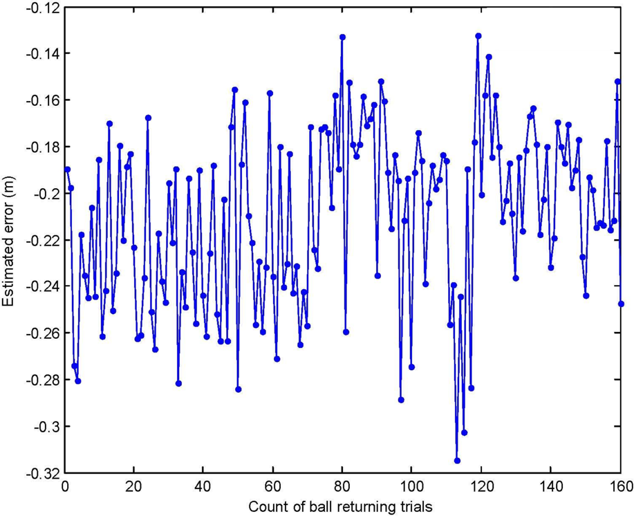
Secondly, error estimation is carried out to obtain landing point error. Figure 8 and Figure 9 illustrate the estimated error of the two groups of ball playing data between a human player and the robot.

Figure 8.

Estimated error for landing point control in Y axis

Figure 9.

Estimated error for landing point control in Y and X axes

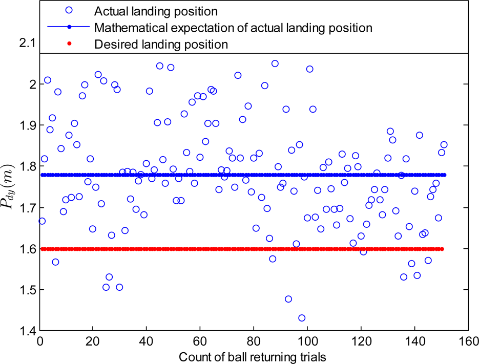
Thirdly, after error estimation results have been obtained, the landing point control method is applied to the robot for competitive table tennis playing. In the first group of ball playing experiments (with the error estimation in Figure 8), the error reduction control in Y axis is applied. The experimental results in Figure 10 show that the mathematical average in Y axis of the landing points in Figure 10 is 1.7795m, and the standard deviation in Y axis is 0.1304m. We can see that the average is 0.1032m less than that in Figure 7, which means that the landing point control method is effective in reducing landing error.

Figure 10.

Landing points distribution when error control in Y axis is used

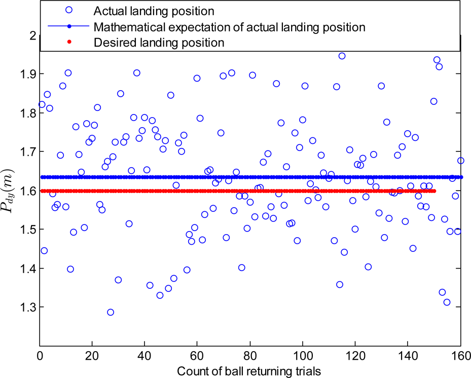
Fourthly, it is clearly that landing point control in Y axis only is not enough to land the ball with a small error. This can be attributed partly that there is a limit for the error reduction control method along each axis. Considering that the velocity V _outx also exerts effects on the flying distance of the returning ball, it can not be neglected in the velocity compensation procedure. In the second group of the ball playing experiments (with the error estimation in Figure 9), Δ V _outx is generated to reduce the landing error of the returning ball. Figure 11 illustrates the actual landing point positions after the error reduction based landing point control in both Y and X axes is used. The results show that the mathematical average of the landing points of the returning ball is 1.6338m, and the standard deviation is 0.1446m. We can see that the average of the landing points has approached the desired position 1.6m with an error of 0.0338m, which is much smaller than the error 0.2827m when there is no landing point control.

Figure 11.

Landing points distribution when error control in Y and X axes is used

Through the experiments, we can see that our methods are effective in reducing the average error between the desired landing points and the actual landing points. However, we should also point out that our method has paid no attention to reducing the standard deviation.

6. Conclusion

This paper has discussed two basic but important issues for competitive table tennis playing, including designation of a landing point and precise landing point control. The work can be summarized as follows.

A landing point designation method is proposed to decide the various desired position of the returning ball according to an expected competitiveness index.

A learning based landing point error control method using the historic playing records is proposed to reduce the error between the actual and desired landing points of the returned balls.

Experiments on the physical humanoid robot have demonstrated the effectiveness of the proposed methods.