
Abstract
Variable-geometry truss (VGT) can be used as joints in a large, lightweight, high load-bearing manipulator for many industrial applications. This paper introduces the modelling process of a multisection three-degree-freedom double octahedral VGT manipulator and proposes a new point-to-point trajectory planning algorithm for a VGT manipulator with a nonlinear convex optimization approach. The trajectory planning problem is converted to a quadratic convex optimization problem, and if some parameters are appropriately chosen the proposed algorithm is proved to be of global convergence and to have a super-linear convergence rate. The effectiveness of the proposed algorithm is illustrated by numerical simulation.
Symbols
M the actuation plane
l i (i=1, 2, 3) length of the i-th actuator
G i (i=1, 2, 3) the i-th node for the low actuation plane
s VGT mid-plane joint offset
l0 fixed batten length
l cross longeron length
O0 the coordinates of the centre of the bottom plane
O t the coordinates of the centre of the top plane
r the length from O0 to the middle actuation plane along vector
θi(i = 1, 2, 3) the cross longeron face angles
N the length from the midpoint of the three sides in the bottom to G i (i=1, 2, 3)
s i , c i (i = 1, 2, 3)sin θ i and cosθ i
P i , Q i , R i (i = 1, 2, 3) intermediate variables to calculate θ i in inverse kinematic problem
O t i (i = 1, 2…, n)O t of the i -th module in the coordinate system of the i -th module
O i = [O xi , O yi , O zi ] T O t of the i -th module in the ground coordinate system
α i (i = 1, 2…, n) the first deflection angle about y axis of the i -th module
² i (i = 1, 2…, n) the second deflection angle about z axis of the i -th module
T i (i = 1, 2…, n) the transformation matrix of the i -th module
ls i (i = 1, 2…, n) the length of the rod seen as the i -th module of VGT
S t =[Sx t , Sy t , Sz t ] T the ideal position wanted
l b the radius of the obstacle
O b the centre of the obstacle
ls max , ls min the given maximum and minimum lengths of ls i
k i (i = 1, 2…, n) the impact factors of the i -th rod
X the optimization variable of the optimization problem
A i constant matrix used to represent O i by X
f(X) the objective function
g i (X) the i -th constraint function
L (X, λ) the Lagrangian function of the optimization problems
λ = (λ1, …, λ2n+1) T the Lagrange multiplier
g(X) the vector of the constraint function
df the gradient of the objective function f(X)
dg i the gradient of the constraint function g i (X)
H(X) = ∇ g (X) T the gradient of g(X)
∇L (X, λ) the gradient of L (X, λ)
∇ X L (X, λ) the gradient of L (X, λ) about X
∇λL (X, λ) the gradient of L (X, λ) about λ
N(X, A)the Jacobi matrix of ∇L (X, λ)
W(X, λ) the gradient of ∇ L (X, λ)
∇2 XX L (X, λ) the gradient of ∇ X L (X, λ) about X
∇2 f the gradient of the objective function df
∇2 g i the gradient of the constraint function dg i
k the iteration number
z k parameter used in quadratic programming subproblem
p k parameter used in quadratic programming subproblem
ω k parameter used in quadratic programming subproblem
d k d for the k -th iteration
d the optimization variable of quadratic programming subproblem
q k (d) the objective function of quadratic programming subproblem
X k X for the k -th iteration
λ k = [λ k 1 λ k 2, … λ k 2n+1]λ for the k -th iteration
α k the step size for the k -th iteration
d*, λ k *, X* the minimum value for d k , λ k , X k
PΣ(X) the penalty function
Σ the penalty parameter
Σ k the penalty parameter for the k -th iteration
Δ, τ parameters to calculate Σ k
P′ (X k , Σ k ; d k ) the directional derivative of P(X k , Σ k ) along direction d k
ε1 ε2 the parameters used to stop the iteration
ρ the parameter to calculate the sizestep
Er, Ea the relative error and the absolute error of the simulation result
B i , C i , D i , Z matrixes used in the proof for Theorem 1
O zero matrix
I unit matrix
[Z] i the columns from the (3i −2) -th column of matrix Z to the (3i) -th column of matrix Z
Introduction
Variable-geometry truss (VGT) manipulator is a kind of hyper-redundant manipulator with a very large degree of kinematic redundancy. It can be used in the fields of remote, unstructured and hazardous environments such as space, undersea exploration and mining.
The VGT possesses a high stiffness-to-mass ratio and provides both structural integrity and function dexterity. Koryo Miura proposed the concept of VGT in 1984 [1] and several papers discussed the design of different structures for a VGT manipulator, such as Rafael AvileHs's paper in 2000 [2], K. Hanahara's paper in 2008 [3] and Sven Rost's paper in 2011 [4]. In 1991, Frank Naccarato and Peter Hughes began to discuss the kinematic problem of a VGT manipulator [5], and further research on the kinematic problem has been undertaken by Robert L. Williams II in 1994 [6] and 1998 [7], Yao Jin and Fang Hai-rong in 1995 [8] and Regina Sun-Kyung Lee in 2000 [9]. However, these papers are all focused on the forward and inverse problems, and there are few papers discussing the trajectory planning of VGT manipulator with multiple modules.
There has previously been several papers discussing the trajectory planning of hyper-redundant manipulators, including David S. Lees' paper in 1996 [10], Vasily Chernonozhkin's paper in 2006 [11] and Chien-Chou Lin's paper in 2012 [12]. However, these papers are only focused on the trajectory planning problem in the two-dimensional plane of the manipulators. The latest research is focused on three-dimensional hyper-redundant manipulator trajectory planning, including papers by Maria da Graça Marcos in 2010 [13] and in 2011 [14]; Samer Yahya also wrote a paper on trajectory planning in 2011 [15]. However, these papers make the manipulator reach the given point by using an extended Jacobi matrix. On one hand, it greatly increases the running time of the manipulators, but on the other, due to the different structures between VGT and the hyper-redundant manipulators mentioned above, the recursive matrix cannot be applied to VGT.
In this paper, a point-to-point trajectory planning algorithm for a three-dimensional VGT manipulator model is proposed using a nonlinear convex optimization approach. The trajectory planning problem is converted to a quadratic convex optimization problem, and if some parameters are appropriately chosen, the proposed algorithm can be proved to be of global convergence and to have a superlinear convergence rate.
This paper is outlined as follows. In the next section, the kinematic model of a double octahedral VGT manipulator is discussed. Section 3 is devoted to point-to-point trajectory planning for the VGT manipulator, and the simulation result is shown in Section 4. The conclusion is drawn in Section 5.
Kinematic Model of a Double Octahedral VGT Module
In this section, we introduce kinematic problems by using the geometry relationship for the single module of the VGT manipulator. The kinematic problems of a VGT module consist of three subproblems: the forward kinematic problem, the inverse kinematic problem and the extensible kinematic problem. At first, we give the description of the VGT manipulator module.
Description of the VGT manipulator module
In order to explain kinematic problems, at first we should introduce the structure of the single VGT manipulator module.
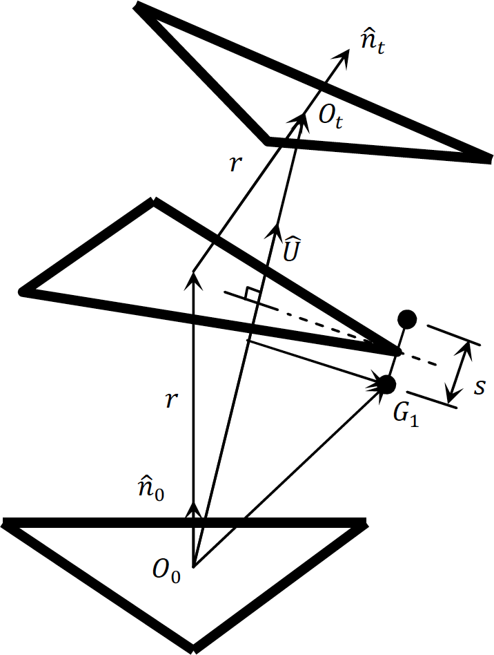
As is shown in Figure 1, a single VGT manipulator module is composed of three kinds of rods: actuators, top and bottom rods and other linked rods. The lengths of the actuators are represented by l i (i = 1, 2, 3) and the actuators' lengths are changeable. We also use l0 to represent the lengths of the rods in bottom plane and top plane and use / to represent the lengths of the rest rods, both l0 and / are constant. The three actuators compose a plane, which is called the actuation plane, and a single VGT manipulator is symmetric about the plane. We use G i (i = 1, 2, 3) to represent the nodes for the actuation plane. In the actual situation, due to the limitation of the mechanical structure, the actuation plane has thickness which is represented by s.
There also needs some other parameters to figure out the kinematic problem. As is shown in Figure 2, we use O0 and O
t
to represent the centre of the bottom plane and the centre of the top plane.

The single VGT manipulator module
Parameters used for the kinematic problem
The other parameters θ
i
(i = 1, 2, 3), which are the cross longeron face angles, are used as the intermediate parameters. We also use N to represent the length from the midpoint of the three sides in the bottom to G
i
(i = 1, 2, 3) and

The intermediate parameters θ i {i = 1, 2, 3)
By using these symbols and the symmetry of a single VGT manipulator module, we will introduce the forward, the inverse and the extensible kinematic problems in the remaining part of Section 2.
For the forward kinematic problem of a single VGT module, the inputs are l i (i = 1, 2, 3) and the output is O t . To realize the process, the cross longeron face angles θ i (i = 1, 2, 3) are used as the intermediate parameters. We use s i , c i to represent sinθ i cosθ i , and by using the geometry relationship of single module and the known l i (i = 1, 2, 3), the intermediate parameters θ i (i = 1, 2, 3) can be figured out by (1) [6],
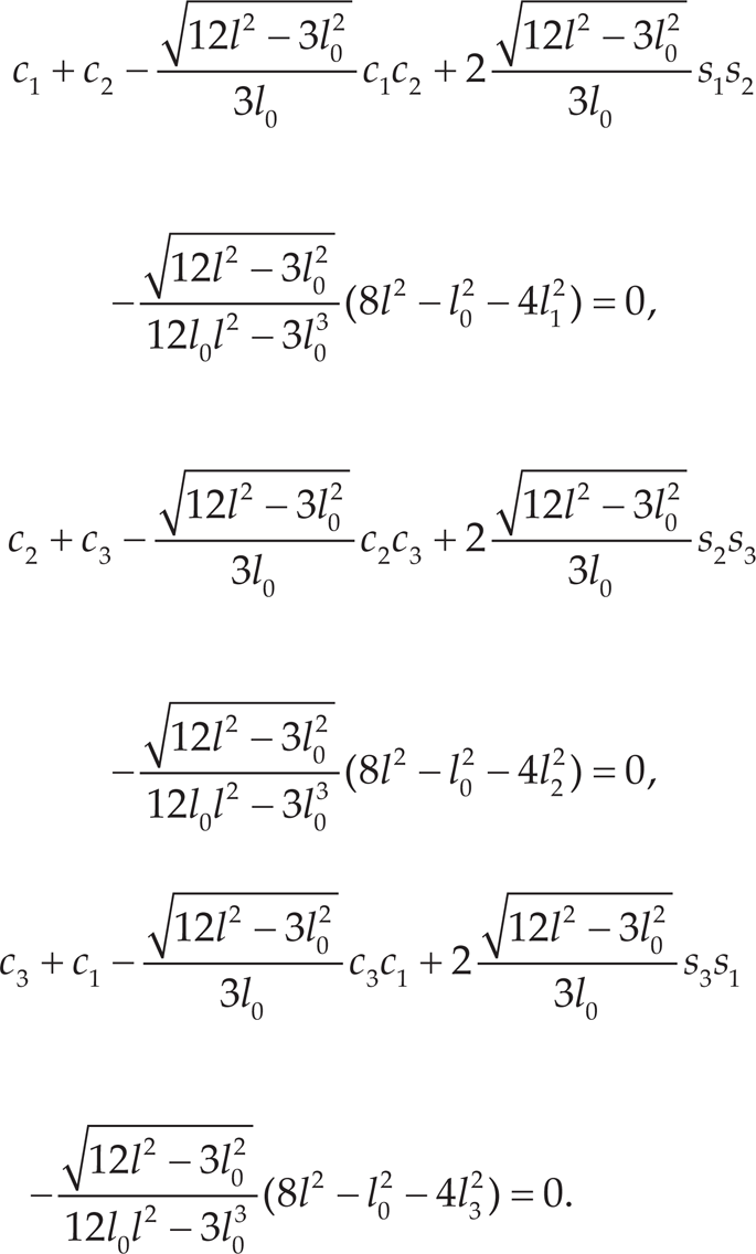
There are eight solutions for θ i (i = 1, 2, 3)in(1), but by taking the actual situation into consideration, one optimal solution for θ i (i = 1, 2, 3) is selected, so θ i (i = 1, 2, 3) are figured out. We realize that for the single module, O0=[0, 0, 0]T, Ot can be calculated with (2–4).


By using (1-4), the forward kinematic problem for the single VGT module is solved.
For the inverse kinematic problem of a single VGT module, the input is O
t
and the outputs are l
i
(i = 1, 2, 3). To realize the process, the cross longeron face angles θ
i
(i = 1, 2, 3) are also used as the intermediate parameters. By considering the relationship of the vectors in Figure 2,

where

where

There are eight different combinations for θ i according to (6), but by taking the actual situation into consideration, there is only one solution left, and by using the solution, G i (i = 1, 2, 3) can be calculated by (4) and then l i (i = 1, 2, 3) is figured out as follows:

By using (4-7), l i (i = 1, 2, 3) can be figured out by O t and the inverse kinematic problem for a single VGT module is solved.
Sections 2.2 and 2.3 discuss kinematic problems for a single VGT module, and this section extends the kinematic problem to multiple VGT modules.
In the calculation of the extensible kinematic problem, we use O
t
i
and

To figure out the transformation matrix for multiple modules, we introduce the new variables α i (i = 1, …, n) and ² i (i = 1, …, n) which are defined in Figure 4 and can be calculated by (8):
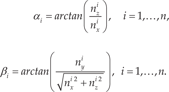
where

Details for extensible kinematic problem

To the forward kinematic problem of the i -th VGT module, we can use l1l2, l3 from the first module to the i -th module to figure out O
t
j
(j = 1, 2, …, i) and

To the inverse kinematic problem for multiple modules, at first we should calculate O
i
(i = 1, 2, …, n) by the given ideal position, and this problem, which is called a point-to-point trajectory planning problem, will be discussed in the next section. After calculating O
i
(i = 1, 2, …, n), we can use them to figure out O
t
(i = 1, 2, …, n) and

Then, by using (4–7), l1 l2, l3 from the first module to the n -th module are figured out, and the inverse kinematic problem for multiple modules is solved.
In this section, we introduce the solution of point-to-point trajectory planning for the n-module VGT with a nonlinear programming approach.
Description of the problem
For simplicity, the i -th module of VGT can be seen as a rod, and the length of the rod is:

The trajectory planning problem can be shown in Figure 5.

Trajectory planning problem with obstacle
If we use S t to represent the ideal position wanted, we can represent the trajectory planning problem as follows,

where ls max and ls min are the given maximum and minimum lengths of ls i and are determined in accordance with module structure parameters via a single module forward kinematic calculation in Section 2, k i (i = 1, 2, …, n) are the weighing factors of each rod and X = [(O1) T , (O2) T , …, (O i ) T , … (O n ) T ] T is the final output.
Assume matrixes A i ∊ R3×3n and
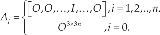
where

Meanwhile


Problem (12) finally becomes
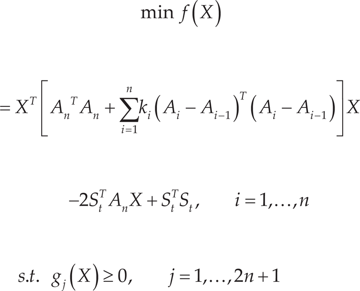
where

Because f(X) and g j (X) are all second-order continuously differentiable real functions, the Lagrangian function of problem (17) is

where λ = (λ1, …, λ2n+1) T is the Lagrange multiplier and g(X)=[g1(X), g2(X), …, g2n+1(X)] T . The gradient of the objective function f(X) is

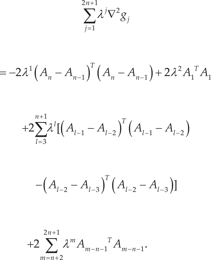
and the gradient of the constraint functions g j (X) are

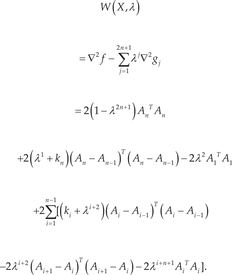
Assume

and according to the Kuhn-Tucker (KT) condition, we have

So, the Jacobi matrix of ∇ L (X, λ) is

where from (18)

and

Then
In general, we use the Newton method to figure out nonlinear equation (21), so to the given point z k = (X k , λ k ), the format for the Newton method is

where p k = (d k , ω k ) satisfies

that is
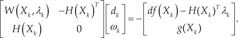
By solving (29), a suitable descent direction can be obtained. In fact, equation (29) can be transformed to a quadratic programming subproblem. Consider the expansions of (29), where

Equation (30) is the KT condition for the quadratic programming subproblem (31) as follows
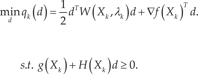
By solving a quadratic programming subproblem (31), we get the minimum point (d*, λ k *). From (30), we can see that d*=d k is the search direction for the k -th iteration of problem (17) and λk+1 = λ k + α k ω k = λ k + α k (λ k * −λ k ) is the Lagrange multiplier for the (k + 1)-th iteration of problem (17) where α k is the stepsize for the k -th iteration of problem (17).
The search direction d k calculated by (31) is used to be the descent direction of penalty function (32),
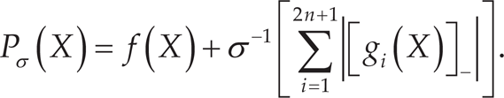
where [g i (X)] = max{0, -g i (S)} and penalty parameter Σ>0. The penalty parameter Σ is obtained by the following rules

where Δ > 0 is a constant and τ = λk∞.
Now use λ k =[λ k 1, λ k 2, …, λ k n+1] to represent the Lagrange multiplier for the k -th iteration and use P′ (X k , Σ k ;d k ) to represent the directional derivative of P(X k , Σ k ) along direction d k . Then, the point-to-point trajectory planning algorithm is shown as follows.
The global convergence of Algorithm 1 is given by the following theorem.

Algorithm 1 is of global convergence.
To make W(X k , λ k ) easy to check in practice, a sufficient condition for global convergence of VGT trajectory planning is given by the following theorem.

Problem (17) is of global convergence.
For the convergence rate of Algorithm 1, we have the following theorem.
Simulation of trajectory planning with an obstacle for three-module VGT is shown in this part. The initial parameters needed are shown in Table 1.
We use [Ox3, Oy3, Oz3] to represent the coordinates of O3 and use [Sx t , Sy t , Sz t ] to represent the coordinates of S t . Then, the relative error Er is calculated by

And if Sy t =0, make (Oy3-Sy t )/Sy t =0. The absolute error Ea is calculated by

Initial Parameters for VGT
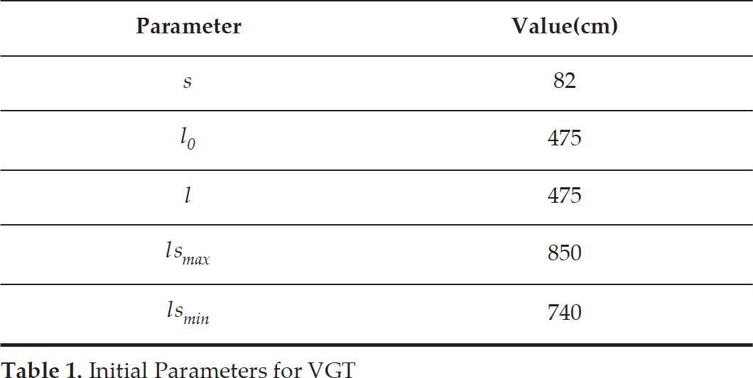
Initial Parameters for VGT
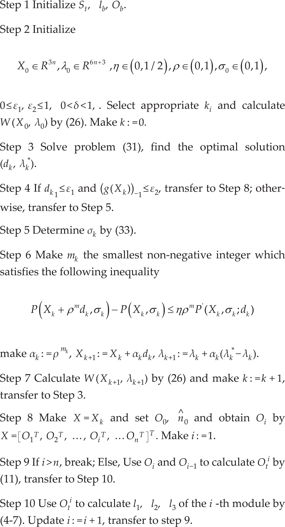
According to Algorithm 1, the steps of the simulation for a single point S t =[2433, −85, 100] T are shown as follows.
Step 1 Initialize

Step 2 Set

Δ=0.05, k i = 0.01 and calculate W(X0, λ0) by (26). Make k: =0.
Step 3 Solve problem (31), find the optimal solution (d k , λ k *).
Step 4 If dk1 ≤ε1 and (g(S k ))−1 ≤ε2, transfer to Step 8; otherwise, transfer to Step 5.
Step 5 Determine Σ k by (33).
Step 6 Make m k the smallest non-negative integer which satisfies the following inequality

Make
Step 7 Calculate W(Xk+1, λk+1) by (26) and make k:=k + 1, transfer to Step 3.
Step 8 Set

Make i:=1.
Step 9 If i > 3, break; Else, Use O i and Oi−1 to calculate O t i by (11), transfer to Step 10.
Step 10 Use O t i to calculate l1 l2, l3 of the i -th module by (4–7). Update i:=i + 1, transfer to Step 9.
To demonstrate the effectiveness of the proposed method, we choose ten different S t in the simulation. The simulation outputs are calculated by (1-4, 10) and the results for ten points are shown in Table 2, Figure 6, Figure 7 and Figure 8.
Results for simulation

From the simulation result, the relative error is 0.54% and the absolute error is 8.15218mm. The simulation is run on a TIP computer with a Core2 Duo 2.93-GHz CPU running the Windows 7 operating system and the software Matlab 2013b. For Algorithm 1, the average running time is 0.233s.

The x-axis position results

The y-axis position results

The z-axis position results
The point-to-point trajectory planning for VGT is discussed in this paper. A new fast trajectory planning algorithm for a VGT manipulator via convex optimization is proposed. The trajectory planning problem is converted to a quadratic convex optimization problem, and if some parameters are appropriately chosen, the proposed algorithm is proved to be of global convergence and to have a superlinear convergence rate. Simulation results in Section 4 show that the proposed algorithm is effective for the trajectory planning of VGT.
Footnotes
Appendix A
The proof for Theorem 1 is shown as follows.
Assume Algorithm 1 is not convergent, K0 is then an infinite set. Without loss of generality, we may assume
According to Temma 2.1 in [18] and the positive definiteness of W(X k , λ k ) given in (34), for each k, there exists a d k for subproblem (31).
then from (29), we have
which satisfies the KT condition of (17). Therefore, by considering the positive definiteness of W(X k , λ k ) given in (34), Algorithm 1 is of global convergence [19, Section 7.7] which contradicts the assumption.
So, we have
where η1 is a constant. According to [18, Temma 2.3, equation 2.13], there is
According to the continuity of PΣ(X), P′(X
k
, Σ
k
; d
k
) is bounded, so there exist
To every iteration, there exists a constant
Since
Appendix B
The proof for Theorem 2 is shown as follows.
where
Here we introduce [Z] k to represent the columns from the (3k−2) -th column of matrix Z to the (3k) -th column of matrix Z, and we use O to represent the zero matrix and I to represent the unit matrix. From (13), is
So, the columns of [Ak1 + Ak n ] are shown as follows
The columns from the third column of [Ak1 + Ak n ] to the (n−2) -th column of [Ak1 + Ak n ] are zero matrix, and
The columns of [D i ](i=2, …, n −1) are as follows
The other columns of [D
i
](i=2, …, n −1)
So, the columns of [W(X, λ)/2] are as follows
According to Gershgorin's disc theorem [20], we can see λ i which are the eigenvalues of any matrix Znxn satisfy
where a ii are the diagonal elements of matrix Z and a ij are the non-diagonal elements of matrix Z. So, we have
So if λ i satisfy
equation (46) is satisfied. Therefore, if
by combining (47) and (48), we will have λ i >0, which means the matrix Znxn is positive definite. Therefore, equation (48) can be used as a criterion for the positive definiteness of a matrix. To make W (X, λ) positive definite, we substitute the elements of W(X, λ) to (48), and then equation (35) is obtained. According to Theorem 1, Algorithm 1 is of global convergence.
Appendix C
The proof for Theorem 3 is shown as follows.
Similar to the Theorem 3.3 in [21], we assume
Then P k ⋅ H(X k ) T = H(X k ) ⋅ P k =O and P k is symmetrical. From (49), is
The first equation of (51) is obtained by (49); the second equation of (51) is obtained by the condition P k ⋅ H(X k ) T =0; The third equation of (51) is obtained using the Taylor expansion of df(X k ).
By using the third equation of (51) is
that is
When X k → X*, there is
which means
and when X k → X*, there is also
From (49), we also have
The first equation of (59) is obtained by (49); the second equation of (59) is obtained since the direction d k is a solution for an appropriate equality constrained quadratic programming, which means g(X*)=0. The third equation of (59) is obtained by using the Taylor expansion of g(X k ).
By moving -H (X k )[X k − X*) in the third equation of (59) to the left side of the equation we can get
Define
So for ∀ d satisfies G*d=0, we have
Premultiply d T by (64), there is
From (62) and (65), we also have P*d=d and according to the symmetry of P*, equation (66) becomes
If Theorem 2 is satisfied, W(X*, λ*) will be positive definite, so from (67), d = 0. Equation (64) has only a zero solution, which means P*(W(X*, λ*) must be full rank. From (58), we have X k +d k −X*=o(x k −X* X*2), that is
Therefore, problem (17) is of superlinear convergence rate.