
Abstract
This paper presents a strategy to improve the navigation solution of the HRC-AUV by deploying a model-aided inertial navigation system (MA-INS). Based on a simpler three-DOF linear dynamic model (DM) of the vehicle, and implemented through a Kalman filter (KF), the performance of the proposed MA-INS is compared to state-of-the-art solutions based on non-linear models. The model allows the online estimation of the sea current parameters before and during the navigation mission. Qualitative and quantitative evaluations as well as a statistical significance test are performed using both simulated and real data, demonstrating the usefulness of the proposed model-aided navigation.
Introduction
Inertial navigation systems (INSs) have commonly been used as a means of localization for autonomous underwater vehicles (AUVs) [1]. The main disadvantage in the use of an INS (particularly with low-cost sensors) is the error growth in the position estimates due to the dead-reckoning nature of the method [2]. Traditionally, external sensors, such as GPS [3, 2], transponders from a time of flight acoustic navigation method [4], Doppler velocity logs (DVLs) [5, 6], sonar [7, 8] or a camera [9, 10], have been used to aid the solution of the inertial navigator, thus constraining the errors in position estimates. These external sensors have several practical disadvantages, essentially relating to the reliance on external information, such as the reception of satellite transmissions or a reliable and observable ocean floor. One source of information that can assist in the localization of the vehicle without the need for extra additional external sensing lies in the use of its DM. The model of the vehicle is capable of representing the attitude of the system according to the control inputs and the external forces acting on it.
Several vehicle model-aided inertial navigators, through the use of non-linear vehicle dynamic equations, have been reported for aerial vehicles [11, 12] as well as underwater vehicles [13]. In this work, we follow the recent developments of MA-INSs for underwater vehicles based on a three-DOF non-linear model [14, 15] and propose a model-aided inertial navigation strategy based on the linear three-DOF DM for the HRC-AUV (a low-cost AUV under development by the Cuban Hydrographic Research Center (HRC) and the Group of Automation, Robotics and Perception (GARP) [16, 17, 18, 19]). The proposed strategy, within a KF framework, also estimates in real-time the magnitude of the main environmental perturbation, i.e., the sea current.
This work places emphasis on the structure, parametrization and evaluation of the MA-INS strategy. Furthermore, as we are dealing with a linear model and in order to deal with errors due to model simplifications, a method is provided to determine the overall variance of the model (based on an expectation-maximization algorithm).
The paper is organized as follows. Section 2 briefly describes the vehicle. Section 3 summarizes the six-DOF NLDM of the HRC-AUV. In this work, starting from the six-DOF NLDM of the HRC-AUV [18], we derive a three-DOF linear state-space model, the vehicle's dynamic navigation model (VDNM), presented in Section 4. The VDNM is used in Section 6 as the core for the KF-based model-aided navigation. Implemented through a KF, the strategy introduces the expectation-maximization (EM) algorithm for the estimation of the uncertainties matrix associated with the model and the sensor measurement of the system. In Section 6, the online sea current parameters estimate is introduced. In Section 7, the experimental results, using both simulated and real data, are discussed along with an analysis and comparison with state-of-the-art MA-INSs. Finally, Section 8 draws conclusions and outlines future work.
Vehicle structure and mission configuration
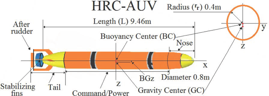
The HRC-AUV is based on the latest design for a submersible vehicle of the Cuban HRC. Developed for supervision and exploration tasks, the design resembles the general structure of several well-known AUVs, such as HUGIN 4500 [14], REMUS [20] and STARFISH [21], but at a different scale and with changes in the governing organs. With steel built in, this low-speed “cigar-shaped” vehicle is completely symmetrical in the x-z plane, with good symmetry in the y-z plane and quasi-symmetric in the x-y plane, as shown in Figure 1. Designed for small depths and medium endurance, the vehicle can operate at depths down to 10 meters for a maximum of 6 hours. The HRC-AUV uses a single main thruster (placed at stern) for propulsion, providing thrust up to 530 N at 24 V and 730 N at 48 V. Its nominal cruising speed is 1.9 m/s at 24 V and 2.8 m/s at 48 V. Steering and depth are controlled by two control rudders also placed at stern and electrically driven.
HRC-AUV mechanical design
The HRC-AUV's geometrical and inertial characteristics are summarized in Table 1 and estimated using the “Mechanical Desktop” software and direct measurements. The HRC-AUV has three basic hull sections consisting on nose, tail and command/power sections. The batteries, based on lead-acid technology, contribute most of the AUVs weight. The batteries are placed at the lower half of the command/power section in order to lower the centre of gravity (GC) and improve roll stability. The vehicle was ballasted to achieve neutral buoyancy.
Geometrical and inertial characteristics of the HRC-AUV

The main onboard sensors are: (i) an attitude heading and reference system (AHRS)(MTi from Xsens [22]), measuring acceleration (fb) angular velocity
The system deploys a navigation/control strategy as depicted in Figure 2. The vehicle can either be remotely controlled (through wireless communication at the surface) or automatically navigate a mission. A mission is parameterized as an initial position, environmental conditions (current direction Bc and magnitude Vc, waves fundamental frequency ωv0), and a set of waypoints to reach. The guidance system computes its current position and, based on it and the position of the next waypoint, provides a reference (heading and depth) that is the autopilot input (updated at each AHRS/INS output). The control, implemented by the autopilot, is based on classical PID controllers for each of the lateral and longitudinal planes [18].

Navigation/Control strategy of the HRC-AUV
In this section, we summarize the six-DOF non-linear DM (NLDM)[18], used to derive the proposed three-DOF linear DM utilized for the model-aided navigation strategy. The six-DOF model has bean developed for the non-linear HRC-AUV simulation [18].
Figure 3 depicts the coordinate systems used in the modelling process of the HRC-AUV along with the definition of the translation and rotation variables of the vehicle. The origin of the vehicle coordinate system, (OB), coincides with the buoyancy centre (BC). Normally, the linear and angular velocities, as well as the forces and moments, are referenced in the vehicle's coordinate system, while the inertial reference system (OE) is used to represent the attitude of the system.

Recommended notation for underwater vehicles [23]
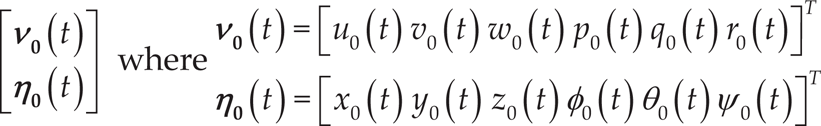
The velocity and attitude vectors are defined as in Equations (1) and (2):


The kinematic relation between the body-fixed velocity v and the position η in the Earth-fixed frame is expressed as follows [23]:
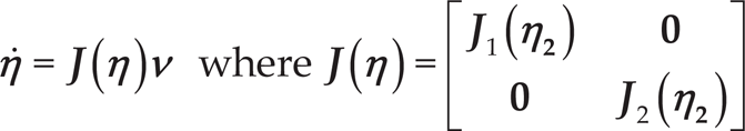


where
The non-linear dynamic equations of motion, including the sea current and waves, can be represented as [23]:

In this structure, M = MRB+MA is the inertial matrix including the added mass,

Here, v is the velocity vector of the vehicle and vc=[uc,vc,wc,0,0,0] T is the current velocity vector, considering that the currents do not generate rotations in the vehicle.
Derivation of the linear dynamic system
As in most of the practical cases, the non-linear equations of motion (Equations (6) and (3)) can be linearized around an operational point [23]. For our case, this point will be defined by:
Since linearization is based on the perturbations from the operational point, such perturbations can be defined as:

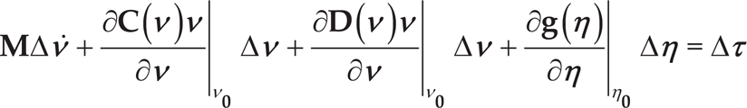
Subsequently, after Taylor series expansion around the operational point, (v0, v0), the equations of motion (6) can be written as:
With the addition of perturbation [23], Equation (3) becomes:

Substituting

where

Establishing x1 = Δν and x2 = Δη, it is possible to present the linear time-varying model of the vehicle:


Where:


Finally, the linear state-space representation of the model can be expressed [23] as:

As such, starting from Equation (17), it is possible to obtain the linear approximation of the vehicle on the longitudinal planes, as made in [24], or else the lateral plane [25].
Due to the operational movement of the HRC-AUV, the heave, roll and pitch can be neglected, such that the characteristics of the vehicle can be achieved through a three-DOF model for the surge motion (advance), the lateral movement in the sway DOF and the yaw angle (heading). At the operational point, the vehicle's travel is characterized by a displacement in the horizontal plane with a heading
Taking into account the above considerations, the operational point is further defined as:

In the same way, the perturbations (Equation (9)) are reduced to:

In addition to the velocity and attitude states, our model considers three complementary state variables describing ocean currents and waves. The current is assumed to be not rotating throughout this work, which implies that each infinitesimal fluid element has zero angular velocity. Following the notation of [23], the current components in 2D can be described by two parameters, namely the average current speed, Vc, and direction of current, Bc:

The average velocity, Vc, can be modelled as a first-order Gauss-Markov process according to:

where wl is a zero-mean Gaussian white noise sequence, and
Waves constitute a problem for surface or near-surface navigation due to the oscillatory behaviour that they introduce. Hence, their modelling allows for the minimizing of their effect through filtering [17]. In this work, first-order wave disturbance, described as a “wave velocity model”, has been considered:


where
Starting from Equation (17) and taking into account the operational point and perturbations (Equations 21, 22), the linear time-invariant state-space representation of the HRC-AUV dynamics is given by Equation (23):

The above equation is referred to as the VDNM. The 9 states, as the representation of the model, depends upon the heading (Ψ0); nevertheless, one can demonstrate that this dependency does not alter the eigenvalues of the matrix A [23]. The matrices in Equation (23) are as follows:

This is because the heading is assumed to be constant at the operational point J* = 0[23].
The discrete representation of the VDNM equation, with the state vector xk = [uL, vL, rL, xL, yL, ΨL, xh1, xh2, Vc], can be easily obtained from Equation (23) by considering the basic characteristics of the operational point, such as the sampling period of the system (dT = 0.01sAHRS sample time), and assuming initial conditions for the heading (ΨL 0 = 0), current magnitude Vc = 0.2 m/s and direction (Bc = 100), and the waves' fundamental frequency (wv0 = 6 rad/s):

with:


the term
The HRC-AUV has been designed to operate in the ocean with a current magnitude not larger than 0.3 m/s and a mean wave height corresponding to sea level 3. These values are in concordance with the physical oceanography of the Cuban maritime platform, where the upper layer circulation is dominated by the Caribbean Current [26]. The sea current magnitudes are taken from Cuban studies on the subject [27]. The HRC-AUV cruise speed for the reported experiments u0 =1.9 m/s is obtained at 24 V, which is approximately 500 rpm of the propulsion engine. This condition only changes due to environmental perturbations because the propulsion engine is directly connected to the batteries without any regulation system (only a controlled switch [19]).
According to the mechanical design of the HRC-AUV, the tail rudder deflection angle is ±30° (Table 1) with a maximal rate of turn of 4°/s. This rate of turn is high in order to obtain the assumed steady-state behaviour during the hardest manoeuvres expected for the vehicle, being a ±90° heading change. From several simulations (like the one presented in Section 7.0.1), it was possible to determine that a reduction of this parameter to only 0.8°/s will ensure the required soft operation. We also established a limit of 100 m between successive manoeuvres in order to allow heading control and to establish the desired course, since the settling time of the system operating at a cruise speed of 2.8 m/s is 40 s, which gives an approximate travel distance of 100 m (valid also for the system operating at 1.9 m/s).
The “operational point” of the HRC-AUV will be changed each time the heading ΨL 0 differs by 6 degrees from the estimated heading ΨL. A new “operational point” is then established, with ΨL 0 = ΨL and updating the angle between the vehicle and the ocean current (Bc − ΨL 0). The value of 6 degrees was selected after several simulations and having conducted several field experiments. Smaller values cause unstable behaviour due to the oscillation introduced by waves, while higher values are demonstrated to affect the performance of the linear model. For these analyses, it was considered that the ocean current magnitude (Vc) and direction (Bc) were constant.
Summary of the HRC-AUV estimated and the identified parameters

Summary of the HRC-AUV estimated and the identified parameters
Table 2 details all the terms used in the VDNM. Several of these parameters were estimated from the vehicle's geometric and inertial data. Others, like those associated with the viscous damping and the control inputs, were estimated through experimental tests; details can be found in [18]. Finally, the general structure of the VDNM model input/output is illustrated in Figure 4.
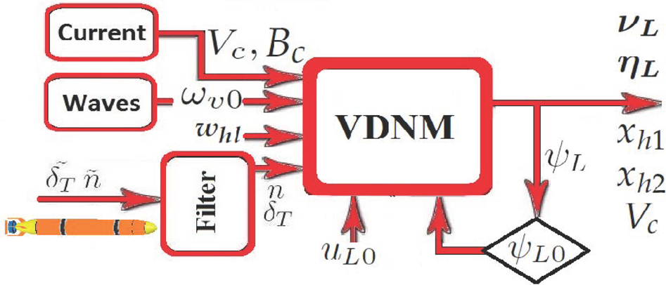
VDNM input/output structure
The primary challenge in AUV navigation is maintaining the accuracy of its position over the course of a mission. AUVs present an uniquely challenging navigational problem because they operate autonomously in a highly unstructured environment where satellite-based navigation is not directly available; hence, they must navigate using other methods when submerged. The most common methods currently used for AUV navigation are INSs and time of flight acoustic navigation.
The deployed inertial solution on the HRC-AUV is presented in Figure 5. In this scheme, the acceleration due to gravity is subtracted from the measurements of the accelerometer (fb) of the AHRS. First, an integration is performed to obtain the velocity

AHRS/INS output
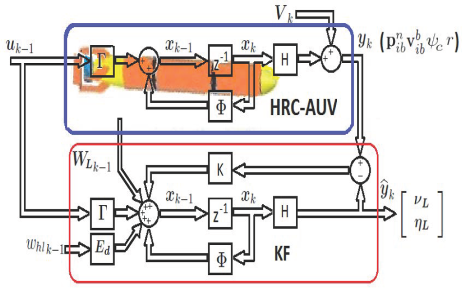
The main disadvantage of INS is the error growth in the position estimates due to the dead-reckoning nature of the method. In this work, we follow the idea and concept of using the dynamic vehicle model for aiding an INS [14, 15]. The use of a vehicle DM as a source of information to aid the solution of the inertial navigator has the benefit of not requiring any additional hardware and the potential of being self-contained. Figure 20(a) illustrates how the output from the model is treated analogously to that of an external aiding sensor. In the proposed configuration of Figure 20(b), the estimated state vector is composed of xk = [uL,vL,rL,xL,yL,ΨL,xh1,xh2,Vc] T , and the process model is expressed according to Equation (24):

Observation is given by:

with:
and V is an uncorrelated, zero-mean observation noise vector of covariance R with a diagonal structure and values according to each manufacturer's specifications.
The sensors installed onboard the HRC-AUV are capable of measuring all the components of the attitude vector
A KF is a good choice for the integration of inertial and DM data under the assumptions of a Gaussian probability distribution (as the outputs of the VDNM and the INS systems are contaminated with noise and uncertain dynamics (
Observer structure
As in any process of modelling a physical system, our final model contains errors in the estimation of several parameters (due to incomplete geometrical data or unknown errors in the experimental data). As such, if we can reflect these errors in the covariance matrices
In this work, based on the recorded trial data, we apply the EM algorithm [31] for estimating the noise covariance matrices

In the second step, fixing the value of

Sea current estimation
As discussed in section 4, the sea current is considered irrotational and as acting on a 2D frame (this is a basic assumption like that which can be found in [34, 15, 35]). The sea current is described by two parameters, the average current speed, Vc, and the direction of current, Bc. For short-term experiments, the direction can be assumed as constant, since the average current speed can be considered to be slowly varying (Equation (21)). The sea current is the main environmental perturbation acting over the AUV's navigation, and an incorrect initialization of the current parameters will affect the DM's performance. To overcome this problem, prior to each mission, it is necessary to conduct experiments for estimating the sea current's characteristics.
Sea current direction estimation
Prior to a navigation mission, an open-loop control strategy is applied to the AUV, in which the vehicle is instructed to introduce a constant rudder deflection angle that provokes a turning manoeuvre. In the absence of a sea current, this type of command will produce an almost perfect circle (Figure 7, red pattern), but in the presence of a sea current a sliding pattern is obtained (Figure 7, blue dashed pattern). The same conditions can be obtained if the commands (n and ΔT) are provided to the DM (VDNM, without sea current initialization) and its position outputs are recorded as well as INS or GPS measurements. From the recorded data, it is possible to estimate the centre of each sliding circle (ci). A least-square line fitting over the centres, ci, allows the estimation of the drift angle introduced by the current.

Simulated experiment for the identification of the sea current's direction
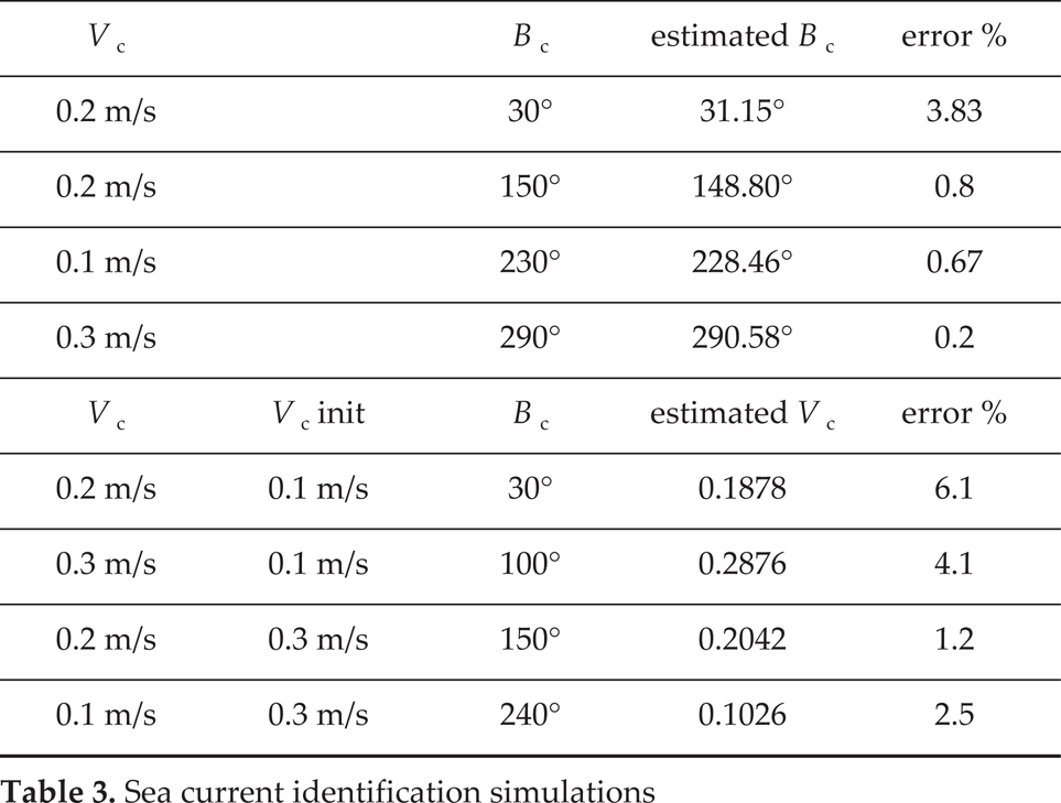
Figure 7 represents simulated experiment that reproduces the above-described conditions (n = 500 rpm, ΔT = 0.45 rad and Bc = 30°). Based on the vehicle speed and manoeuvre strength, a series of position samples are taken (three each time), from which the theoretical centres of the circumferences circumferences are calculated. Since the proximity or distance between points over the arc influences the estimation of the centre, several samples are created with different time intervals between them. Figure 8 illustrates this process and the estimated Bc, showing that, for samples spaced between 10–20s each, the estimated value is quite accurate. Several simulations were conducted with varying sea current speeds (Vc) and directions (Bc), allowing us to validate the presented results (see table 3) with errors smaller than 10% of the true value.

Sea current direction identification
A similar procedure was implemented in real sea manoeuvring conditions (Figure 9). Using the above-described approach, a sea current direction of 219.83° is estimated using GPS inputs, and 229.39° using INS measurements (Figure 10). Knowing that the approximated true value of Bc is 220°, both the Ins and the GPS measurements give the necessary performance to conduct short-term identification procedures like the one presented. It is valid to remark that a low-cost INS decreases performance over time, giving a bigger error than that estimated through the absolute measurements provided by GPS. A similar procedure based on GPS measurements and a least-squares method has been reported in [15, 36].

Sea trial for the identification of the sea current's direction

Sea current's estimated direction
The average current speed is dynamically estimated during navigation, as indicated in Equation 21 and the VDNM model (Equation 24). The observer processes the data from the VDNM and the measurements of the INS in order to estimate the state variable model (Equation 24). The observer processes the data from the VDNM and the measurements of the INS in order to estimate the state variable Vc (average current speed). Figure 11 illustrates the simulated experiment, in which the average current speed is initialized with an incorrect value of Vc = 0.1 m / s instead of the correct value of Vc = 0.2 m / s. As can be seen from Figure 12, the true value is reached very quickly. At the end of the experiment, the mean value is Vc = 0.2053 m / s.

Simulated experiment for the sea current's average speed

Estimated average of the sea current's speed
Several other simulations (see table 3) as well as sea trials (section 7.0.2) were conducted, with different types of manoeuvres and magnitudes of Vc, demonstrated the same behaviour for the correct estimation of the average Vc value.
Sea current identification simulations
To validate the proposed VDNM, two evaluation tests were made. As a first evaluation test, a set of lateral rudder commands (ΔT) are generated to reproduce a desired path; the set is then introduced to the six-DOF NLDM [18] and the VDNM to compare their respective simulated behaviours. In a second validation experiment, both the six-DOF NLDM and the VDNM were provided with the rudder data recorded during sea trials, and their outputs were compared to the sensor readings. Moreover, statistical significance – being an estimate of the degree to which the true position lies within a confidence interval around the GPS measurement was applied using the 2D paired Kolmogorov-Smirnov (KS) test [37].
The (two-sample) KS test statistic measures the distance between the empirical cumulative distribution functions of two samples in order to test whether they have been drawn from the same distribution. The MATLAB implementation that was used includes a parameter α, allowing for the testing of the desired significance level for rejecting the null hypothesis. The outputs of the test are: (a)“pValue”, an estimate for the 'P' value of the test, whereby a large value compared to the selected significance level allows for accepting the null hypothesis; and (b)“KSstatistic”, the KS statistic indicating the distance between the two samples.
Linear dynamic model – first evaluation test
In this simulated experiment, both the six-DOF NLDM and the VDNM models are provided with a set of commands that reproduces a trajectory of 4 km with successive ±90° turns. This type of manoeuvre was selected because it represents the hardest manoeuvre planned during the operation. The rate of turn of the input command was adjusted to only 0.8 ° /s, according to the practical considerations presented in section 4.3. The propulsion system is simulated with a mean value of 500 rpm, a sea current directio of 100° with a magnitude of 0.2 m/s and waves intensity according to sea level 2 (waves height between 0.2 m and 0.5 m) [34].
As shown in Figure 13 and Figure 14, the behaviour of the position output form the linear mdoel degrades over time.

The VDNM and six-DOF NLDM model's position output

The VDNM and six-DOF NLDM model's heading output
This is because each turn causes an estimation error in the VDNM of the speed 13 vector
Figure 15 shows the errors achieved in the estimation of the velocity components of vector
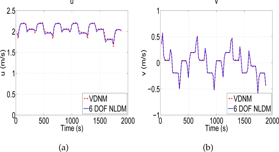
v components
Goodness-of-fit of the VDNM

The second test (Figure 16) represents the responses of the VDNM and the six-DOF NLDM, respectively, using as input parameters (n,ΔT) gathered in a path-following experiment. In this experiment, the HRC-AUV was instructed to start a trajectory at point A and reach points B, C, D and E, separated by approximately 800 m each. The full path describes a trajectory of approximately 3.6 km and a duration of more than half an hour. This path presents a challenge for the VDNM, because throughout it there are several hard manoeuvres (turns at points B and C, both in excess of the suggested 0.8°/s command rate) and full system stops between points B and C. For the evaluation, both models were initialized with a set of parameters that resemble the environmental conditions reported at the test site (the waves' fundamental frequency ωv0, the ocean current direction Bc and the magnitude Vc).

Position estimated by both models vs sensor measurements
Prior to starting navigation, the VDNM and the six-DOF NLDM were initialized with the data of the onboard sensor system: attitude (φ,θ,Ψ) from the AHRS measurements; position (x,y,z) from the GPS; and depth sensor measurements, respectively. After initialization, both models operate using the recorded inputs (in an open-loop scheme). The estimated output positions were compared to GPS measurements in Figure 16 and AHRS heading measurements in Figure 17. While Figure 18 depicts the components of the vector

Heading estimated by both models vs sensor measurements

v components estimated by the models.
As can be seen, the responses of both the six-DOF NLDM and the VDNM are quite consistent with the measurements of the sensors onboard the HRC-AUV. To obtain an evaluation of the precision of both models, we again applied the 2D KS test, looking for the goodness-of-fit between the GPS measurements and the position output of the models. The general measurements characteristics of the Garmin GPS XL-12 onboard the HRC-AUV [16] are presented in Table 5. From these confidence intervals and the well-known Rayleigh distribution of the GPS position measurement, we can infer that its variance is 5.2577m.
Garmin XL-12 measurement performance.

With the information of Table 5, it is possible to test the distance between the empirical cumulative distribution functions (CDFs) of the models' position output and the GPS position measurement. Form Table 6, one can notice that the p-value for the six-DOF NLDM and VDNM is higher than the significance level of our test (α = 0.05); hence, we can conclude that the CDFs of the six-DOF NLDM and VDNM do not differ from the distribution of the GPS position measurement. This result is consistent with the assumed simplifications and the results obtained by simulation in the previous section. Nevertheless, it is possible to assume that the performance level of the linear model in an MA-INS scheme could be improved so as to almost match the non-linear model response for the same purpose by the tuning of the associated covariance noise parameters.
Deploying the data fusion algorithm presented in Figure 6, and using the EM estimated parameters (

Evaluation of the different navigation procedures
Statistical summary of the test

As shown in Table 6, the general navigation performance of the tuned VDNM for MA-INS is similar to the GPS measurements (for short-term missions). It is hoped that a more complete configuration involving the control would increase the performance and robustness of the navigation.
Finally, we compared the proposed MA-INS (denoted by INS+VDNM (optimized)) to the strategy proposed in [15] (denoted by INS+3-DOF NLDM). Both strategies are illustrated in Figure 20. The strategy proposed in [15] deploys an extended KF (EKF) to estimate the errors in the INS outputs from the measurements provided by the model speed outputs. Following the equation set in [15], the six-DOF NLDM presented in section 3 is reduced to a three-DOF NLDM (see [18] for the detailed equations) and used as model for the INS+3-DOF NLDM strategy. It should be noted that the difference between the two strategies is that the VDNM provides an estimate of the attitude of the system that is used in the correction process. Furthermore, for the proposed configuration, the VDNM constitutes the core of the observer, while in the alternative structure of [15] this role is played by the INS.

High-level model-aided INS outline. (a) Strategy proposed in [15] (b) Our proposed strategy.
Figure 21 and Table 6 summarize the comparative results of the two strategies.

Evaluation of the alternative aiding procedures
As can be seen, the two strategies obtain similar results, namely slightly better results are achieved with the proposed IN INS+VDNM (optimized) approach (for the available experimental data). The increase of pValue and KSstatistic indicate that the curve generated by the INS+VDNM (optimized) better approximates the GPS samples. This is due to the adjustment of the parameters associated with the model and measurement uncertainties.
We proposed in this work an accurate linear dynamic model (i.e., the VDNM) for the HRC-AUV. The proposed linear model is used to deploy an MA-INS through a KF. Moreover, an EM algorithm along with Kalman smoothing was used to obtain the covariance matrices of the process and the measurements. The proposed observe, in combination with a set of manoeuvres prior to mission, allows for the embedded real-time estimation of sea current's average speed. The use of the linear model's assistance is shown to be an effective approach, increasing the level of autonomy and robustness of the system. Comparisons with state-of-the-art model-aided navigation showed that our proposed solution allows obtaining similar navigation performances with a less complex model. The general field evaluation of the proposed strategy showed that it is a viable solution. Furthermore, since it does not require any additional instrumentation, it is a good engineering solution to improve HRC-AUV navigation. In addition, being the VDNM a linear state-space model, a wide variety of control strategies and data fusion techniques (not addressed in this document) are now available to enhance the overall performance of the AUV.
Footnotes
9.
This work has been partially supported by the Flemish Interuniversity Council-University Cooperation for Development (VLIR-UOS) within the IUC-UOS project with the Universidad Central “Marta Abreu” de Las Villas (UCLV).