
Abstract
Previous research dealing with constrained kinematic redundancy problems focuses on manipulators with time-independent constraints. This paper extends the general-weighted least-norm (GWLN) method to manipulators with time-dependent constraints by introducing time-dependent virtual joints. In the virtual joint space, corresponding task space velocity is revised to encapsulate the effects of time-dependent parameters of constraints. This is done so that an intermediate kinematic control problem with only joint limit is obtained. Then, the inverse kinematic problem is solved in the virtual joint space. A new inverse-weighted matrix setting criterion is proposed to replace the one-step prediction that originally complicated implementation of the GWLN method. To demonstrate the efficacy of the method, simulations and experiments are carried out on a five-link welding manipulator to track the welding trajectory. Time-dependent orientation constraint and preventing joint limits is guaranteed using this method.
Keywords
1. Introduction
In comparison to non-redundant manipulators, redundant manipulators have greater flexibility and dexterity in motion [1, 2]. For kinematically redundant manipulators, there are infinite solutions in the joint space for tracking a desired end-effector trajectory, which is referred to as the main task. In order not to affect the motions of the main task, redundancy in the main task can be used to obtain a solution simultaneously while performing other subtasks. These are usually formulated as constraints, such as joint limits or obstacle avoidance, and are called constrained kinematic redundancy problems [3].
A large body of research has appeared in the literature regarding control strategies, which effectively exploits the potential advantages of kinematically redundant mechanisms to achieve subtasks. The gradient-projection method (GPM) is a widely used method. A quadratic cost function to relate subtasks is presented. Joint motions are obtained without deteriorating the main task. This is achieved by projecting the gradient of the cost function onto the null space of the Jacobian matrix, which is the quickest decreasing orientation for the cost function [4, 5]. Mansard and Chaumette presented a directional GPM used to cast the gradient vector of the subtask into a space, which accelerated the convergence of the main task [6].
The task-priority framework was addressed based on GPM. The main task and constraints were typically classified into two distinct levels. The lower level task was realized in the null space of the higher task [7]. Then, the method was extended to any number of priority levels [8]. A unified method for unilateral constraints was proposed in [9], and a varied weights method was proposed for the kinematic control of redundant manipulators with multiple constraints [10]. In particular, a quadratic program solver was used to deal with a task-priority problem with inequalities in [11, 12].
Alternatively, constrained kinematic redundancy problems can be considered as a quadratic programming (QP) problem. Compact-Inverse QP method and duality theory are introduced to simplify the QP problem [3, 13]. At the same time, a primal-dual neural network based on linear variational inequalities (LVI) has been used to solve the QP problem [14–16]. A minimum-velocity-norm (MVN) scheme based on a primal-dual neural network has been presented to solve the QP problem with a minimumvelocity solution satisfying constraints. The MVN scheme has been used to successfully resolve the robotic redundancy problem with inequality-based obstacle avoiding tasks [17, 18]. However, solutions generally are computationally intensive.
Chan and Dubey proposed the weighted least-norm method (WLN) for joint limits avoidance [19]. A larger efficiency was demonstrated towards the utilization of redundant degrees of freedom (DOFs) in comparison to GPM. This is because the method preplans no motion for the subtask but does not allow any motion to violate the subtask. To deal with constraints other than joint limits, the general-weighted least-norm (GWLN) method was proposed in [20]. In GWLN, a homogeneous transformation is used to map the actual joint space to a virtual joint space, and the virtual joints with joint limits are used to present the constraints. Using the weight factor setting rule with one-step prediction, the constraint was satisfied by applying the WLN method on virtual joints.
The research focus has been limited to controlling redundant manipulators under time-independent constraints, such as joint limits and obstacle avoidance. However, in practice there are cases with time-dependent constraint, for example, end-effector of the manipulator tracks a trajectory, while avoiding a moving obstacle.
Another example of time-dependent constraint is welding torch orientation constraint in welding process control. In welding process control, the manipulator is required to simultaneously get the end-effector to track the welding seam and keep track of the orientation of the welding torch to satisfy constraints, which guarantee welding quality.
The usual strategy is to take welding process control as a five DOFs task, which includes three DOFs for position task and two DOFs for orientation [21, 22]. In this paper, welding process control is realized by simultaneously performing a three-dimensional position task with a welding torch orientation constraint. The orientation is defined by the intersection angle α between the preplanned desired welding torch direction vector Od and actual welding torch direction vector Oa, which is smaller than the threshold angle β. Both Od and Oa are three-dimensional unit vectors. As shown in Fig. 1, Oa is in the inner of the right circular cone, whose axis is Od and apex angle is 2β. Thus, additional redundant degrees of freedom are obtained to do other tasks, such as joint limit avoidance. Actual orientation Oa is determined by joint position, while the desired direction Od is usually decided by the desired position of the end-effector. Since it is difficult to describe the complicated welding trajectory using an analytic expression, which is a function of position, the preplanned end-effector trajectory is usually represented as a function of time. Thus, the desired orientation Od is time-dependent. Welding orientation constraint can be formulated as

Relation between actual and desired welding torch direction. Here, α is the intersection angle between preplanned desired welding torch direction Od and actual welding torch direction Oa and β is the maximum acceptable deviation angle.

Eq. (1) is a time-dependent constraint.
A majority of the methods discussed previously for problems with time-independent constraint probably cannot deal with time-dependent constraints. A small proportion of the methods consider the constrained kinematic redundancy problem as a dynamic-system-based QP problem, which are available for time-dependent constraints. The MVN scheme falls into this category of methods. However, as stated before, these are computationally intensive.
Here, the GWLN method, which inherits the advantages of the WLN method, is extended to make it applicable for the constrained kinematic redundancy problem with time-dependent constraint. The transformation from virtual joint space and actual joint space is non-homogeneous for a case with time-dependent constraint. Task space velocity is modified to guarantee homogenous transformation. The WLN method can then be applied on the virtual joint space to guarantee time-dependent constraints.
In addition, improvements to the GWLN method are proposed. This is achieved by setting the inverse-weighted matrix to guarantee joint velocity in a continuous manner instead of using the 0–1 switching law [20]. This relaxes the one-step prediction requirement to set the inverse-weighted matrix factors.
The paper is organized as follows: The GWLN method for the inverse kinematic problem with time-independent constraints is reviewed in Section 2. In Section 3, the problem with time-dependent constraint is formulated and the inverse kinematic problem with a single time-dependent constraint is solved using GWLN. The result is then extended to multiple time-dependent constraints in Section 4. The performances of the GWLN method and MVN scheme on welding process control with the time-dependent orientation constraint are compared in Section 5. In addition, experiments on a five-link welding manipulator using the proposed GWLN method are also presented in Section 5.
2. Kinematics control with time-independent constraint and the GWLN method
2.1 Constrained kinematic redundancy problem with time-independent constraint
For a manipulator, relationship between end-effector velocity ẋ d ∈ ℝ and joint velocity q̇ ∈ ℝ n can be represented as:

where J is the m×n Jacobian matrix. In this paper, a situation where n>m is considered, which means redundant DOFs are available to deal with subtasks in the application. A general subtask is represented in the form of an inequality:

where Hg (q) is the time-independent constraint function, hgl is the lower bound of the constraint.
2.2 Review of the GWLN method
GWLN method was proposed to solve Eq. (2) under Eq. (3) in [20]. GWLN takes Hg (q) as a virtual joint variable. To map the real joint velocities into virtual joint velocities, a coordinate transformation matrix T is used and given as:

where

Kinematic control equation in a virtual joint space is:

where Jv=JT−1 is the virtual Jacobian matrix. Virtual joint velocity is determined by:

where Wv −1 is inverse-weighted matrix, defined as:

By setting the corresponding weighted factor, virtual joint motion will be suppressed as it reaches a predetermined limit. In the presence of only one constraint defined in Eq. 3, all diagonal elements are set as 1 except for w̄v1, which is defined as follows:

where ε is a positive scalar defining a safety region length.
Closed loop solution to (2) under constraint defined by Eq. (3) is:

where ke is the feedback gain, and e is the tracking error. The tracking error is defined as:

In practice, there are two problems with the weights setting law in Eq. (9): First, a sign of virtual velocity q̇v1 should be known beforehand to set the value of w̄v1, but the latter decides the former. Second, switch of w̄v1 leads to discontinuity in q̇v1. To solve these problems, a one-step prediction along with a low-pass filter on w̄v1, was proposed for setting w̄v1 in [20].
3. GWLN method for time-dependent constraint
3.1 Time-dependent constraint
Here, we assume that a general time-dependent constraint on the manipulator can be formulated in the form of bilateral inequality with time-variant parameters, that is:

where Hg(q,k):ℝ n × ℝ l ↦ ℝ is the time-dependent constraint function, k ∈ ℝ l is a time-variant parameter, l is the number of time-variant parameters, hgl is the lower bound of the constraint, and hgu is the upper bound of the constraint. One simple case is when k = t. The problem is to find the inverse kinematic solution to Eq. (2), which is subjected to constraints defined in Eq. (12).
3.2 GWLN method solution for time-dependent constraint
For time-dependent constraints, besides the transformation matrix T, an extra transformation matrix M is added as:

where Nq∈ℝ(n-1)×n is the same as defined before.
The virtual joint velocity q̇ v and virtual joint kinematic equation are described as:


Both transformations from the virtual joint space to the task space and from the joint space to the virtual joint space are non-homogeneous. The weighted technique defined in Eq. (9) is not able to guarantee that the virtual joints satisfy their limits. Due to this, task velocity needs to revised to keep the transformation from the virtual joint space to the task space homogenous.
Kinematic equation on virtual joint velocity can be rewritten as:

where Jv=JT −1 is the virtual Jacobian matrix with respect to the virtual velocity, and
Virtual velocity can be obtained by referring to the GWLN method for time-independent constraint, as follows:

where Wv−1 is the inverse-weighted matrix defined in Eq. (8) and Eq. (9). Note that since solution in Eq. (17) only relates to the inverse matrix of the weighted matrix, Wv−1 can be directly defined to avoid calculating the inverse of Wv as in the GWLN method. Since, one-step prediction to set weight factors [20] is complicated for calculations, a new method is proposed for setting diagonal elements of Wv −1.
A performance function for avoiding virtual joint limits was proposed by Zghal et al. [5] and is given as

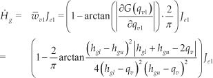
Since w̄v1∈(0,1], the weighted law proposed in [19] is invalid. The following weighted law for w̄v1 is deduced

where
When the virtual joint moves towards its limits, w̄v1 will decrease. This gradually suppresses virtual joint velocity q̇ v1 and eventually the first virtual joint will stop before it reaches the limit (proved in Section 3.3). As the main task moves on, the component of end-effect velocity cast into the first virtual joint direction may change the sign, causing it to move away from the limit. As a result
Eq. (18) is the performance function for a bilateral time-dependent constraint. For a unilateral constraint represented by Hg(q,k)≥hgl, the criterion for deducing weighted factor w̄v1 is defined as:
where δ is a small positive scalar. Then, Eq. (19) can be applied to set the inverse-weighted matrix Wv−1.
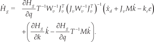
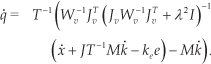
Based on the previous result, the closed-loop control law for Eq. (2) with constraint defined in Eq. (12) is given as:


where (J vw)+=T−1(Wv−1JvT (JvWv−1JvT)−1), and P=T−1Wv−1JvT (JvWv−1JvT)−1Jv−T−1, satisfies JP = 0, is the projection operator onto the null space of the matrix J. GWLN solution to the problem with time-dependent constraint consists of two parts. The first part of Eq. (22) is the same with the GWLN method solution used to a problem with time-independent constraint, provided that the parameter is not time varying. The second part is the projection of the main task onto null space. This is done to overcome the effect of the time varying parameters on the subtask, which does not deteriorate the main task. Eq. (10), obtained from [20], can be regarded as a special case of Eq. (21), provided that k̇ = 0.
3.3 Performance analysis
Definition of the control law given in Eq. (21) and the associated weight setting criterion in Eq. (19) lead to the following theorem.
Proof. Substitute Eq. (21) into Eq. (2), we get

This guarantees that the main task tracking error asymptotically converges to zero. □
On the other hand, more attention is drawn on whether the constraint will be broken, when the weight setting criterion Eq. (19) is applied. In [20], the weight setting law defined in Eq. (9) sets w̄1=0, which directly stops the virtual joint motion approaching the limit to guarantee the constraint. Here the weight setting law in Eq. (19) defines w̄1 close to but not equal to 0. Before to show the compliance of constraints, the following lemma is presented firstly.
Proof. Construct function F(t)=ektu. There is

This demonstrates F(t) is a monotonously increasing function. Referring to u(t0)>0, there is F(t0)>0. Thus, u(t)>0, when t≥t0. □
Proof. For the time-dependent constraint function there is:
According to the definition of matrix T,
Therefore, the second term on the right side of Eq. (25) is always equal to zero and the first term on the right side of Eq. (25) can be simplified as:

Below the method of reduction to absurdity is adopted. Without loss of generality, Hg is assumed to fall below the lower threshold, which breaks the constraint, that is, H=hgl at t = t0. Then, a small time interval [t0-ε,t0] can always be found, where Hg monotonically decreases from Hg| t =t− ε∈(hgl,(hgl+hgu)/2) to hgl at t = t0, and ε is small enough to guarantee 0<(Hg-Hgl) | t0-ε≤1. There is:
where Je1 is the first element of JvT(JvWv−1 JvT)−1(ẋd + JvMk̇-kee). To simplify Eq. (27), middle variables r = qv-hgl and L =hgu−hgl were defined. There is:

Referring to the property of inverse trigonometric function,

For the matrix (JvWv −1JvT) is full rank, JvT (JvWv −1JvT)-1 is bounded, JvT(JvWv −1 JvT)−1(ẋd+JvMk−k̇ee) is also bounded. Thus, there exists a constant scalar φ such that ‖Je1‖ ≤ φ, when t ∈ [t0-ε,t0]. According to r is monotonically decreasing, when t ∈[t0-ε,t0], there is 0≥Je1 ≥−φ,
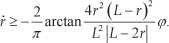
Since, Hg|t=i0−ε<(hgl+hgu)/2 and Hg is monotonically decreasing, L−2r>0 holds, t ∈[t0−ε,t0]. Thus:
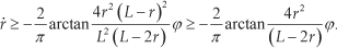
Referring to arctanx≤x, if x≥0 and r≤1, there is,

Since, 8φ/(π(L−2r |t0−ε))>0 and r (t0−ε) >0. Lemma 1 leads to the conclusion r(t)>0, as t ∈[t0−ε,t0]. This contradicts the assumption that r(t0)=0. This implies that the time interval, at which the performance function Hg falls to hgl, does not exist. This shows that Hg>hgl under control law defined in Eq. (21). Similarly, it can be shown that Hg<hgu. □
The aforementioned proof clearly shows that the control law in Eq. (21) and the associated weight setting criterion in Eq. (19) guarantees time constraint and allows a more strict result such that H(q,k) satisfies hgl<H (q,k)<hgu. If the constraint is unilateral, then the proof is perfectly analogous.
Compared with the weight setting criterion defined in Eq. (19), Eq. (9) sets w̄v1=0 at the virtual joint limit. This directly stops any motion of the related virtual joint. However, this criterion also locks the virtual joint as the virtual joint reaches the joint limit. Allowing the virtual joint to quit the limit is another reason to introduce one-step prediction. On the other hand, the weight setting criterion in Eq. (19) keeps the virtual joint within a feasible range, while the joints have not reached the virtual joint limit. This guarantees that w̄v1>0 always holds. Thus, the situation where the virtual joint can get locked is completely avoided.
The damping factor λ is determined according to [23].

where σm is the minimal singular value, ρ is a positive constant, which defines the size of the singular region. λmax is the maximum value of the damping factor. It should be pointed out that the damping factor λ≠0 and tracking error does not asymptotically converge to zero. This will deteriorate main task precision. Although JvWv−1JvT is not full rank, JvT (JvWv −1 JvT + λ 2 I)−1 is still bounded. For control law defined in Eq. (28), theorem 2 still holds.
4. Inverse kinematics under multiple constraints
In this section the results from the previous section are extended to the case of multiple subtasks. This includes both time-dependent and independent constraints. Without loss of generality, it can be assumed that there are r time-dependent constraints. A time-independent constraint can be considered as a special case of time-dependent constraint as stated in Remark 1. Multiple time constraints are formulated as follows:

k ∈ ℝ l is a time-dependent parameter, l is the number of time-dependent parameters. Hgi is the i th constraint function, hgiu and hgi l upper threshold and lower threshold of the i th constraint, there must be r≤n; or else constraints can be combined into one constraint. This method to combine multiple constraints into a single constraint has been discussed later in this section. Virtual joint velocity can be defined as follows:

T and M matrices are defined as:

where Nq ∈ ℝ(n −
r
)×
n
is composed of unit orthogonal vectors, which satisfies
Correspondingly, the inverse-weighted matrix is defined as:

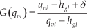
where G(qvi) is the performance function defined in Eq. (18). If the constraints are unilateral, performance functions follow the definition in Eq. (20) and the solution is the same as Eq. 28. Corresponding to proofs for the case with a single time-dependent constraint system, Theorem 1 and Theorem 2 can be easily extended to the case with multiple constraints.
For (n−m) diagonal elements of Wv−1 are near zero and Jacobian matrix J is full rank. Matrix JvWv 1 JvT can still be full rank. If JvWv−1 JvT is singular, the damped least-square technique can be used.
For the case where the number of the time-dependent constraints is higher than the number of DOFs of the manipulator system, the strategy proposed in [20] is used here. For this case, several constraints that cannot simultaneously converge to their limits are merged into a new compact constraint Hc (q, k) as follows:

where Hgi (q, k) is the i th original constraint function. G is the performance function defined in Eq. (18) or Eq. (20), and Φ denotes the index set composed of constraints, which are not triggered simultaneously. μ is the threshold of compact constraint. The compact constraint can be treated as a normal constraint within the GWLN framework.
5. Application to welding control
Here, the GWLN method is applied to industrial welding control to verify efficacy. In this paper, the welding task is realized by performing a three-dimensional position task with a welding torch orientation constraint, shown in Eq. (1). In Eq. (1), Od is time-dependent welding torch direction, pipe-to-pipe intersection seam welding task is selected as an example to illustrate the selection method for Od. The entire welding seam is composed of segments
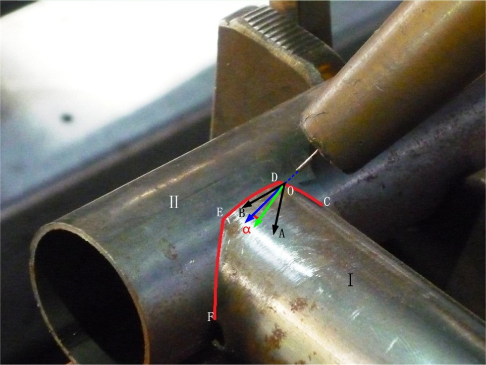
Pipe-to-pipe intersection seam welding task with orientation constraints. Red line represents intersection line of the pipes to be welded. The green arrow represents the desired torch direction Od at an instantaneous moment, and the blue arrow represents the actual torch direction Oa.

where point O is actual position of end-effector at any selected moment.
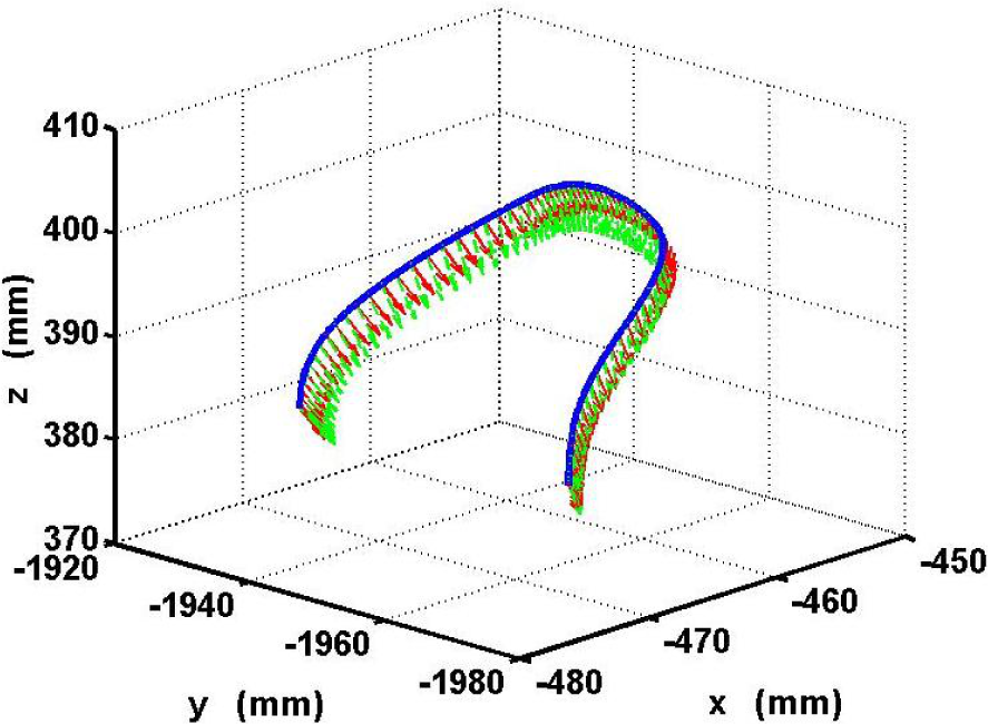
End-effector trajectory under GWLN method, green arrows present the desired welding torch directions, red arrows present the actual welding torch directions under the GWLN method

A welding control problem can be treated as a kinematic problem with time-dependent constraints.
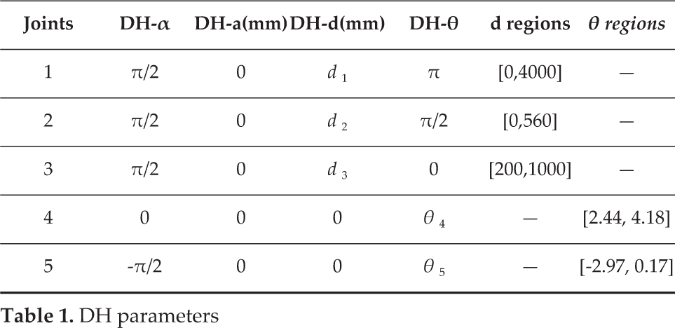
Simulations were carried out by applying the GWLN method to ZT-010 welding manipulator. The manipulator has five DOFs and was designed by Zhejiang Zhengte Group Co., Ltd and Zhejiang University for welding pipe-to-pipe intersection seam of fences. The welding manipulator has five joints. There are three prismatic joints near the base and two revolute joints at the end, as shown in Fig. 4. Danavit-Hartenberg (DH) parameters and limits for the joints are listed in Table 1. Pose and position of the end-effector at the last joint coordinate are PE 5=[87,0,147] T and OE 5 = [−sin(π/6),0,cos(π/6] T .
DH parameters

Five-link welding manipulator
5.1 Simulation result
5.1.1 GWLN method
In this section, simulations based on the five-link welding manipulator for welding control are carried out to verify efficacy of the proposed GWLN method.
The GWLN method was simulated on the five-link welding manipulator for welding control The end-point of the welding torch should track the. pipe intersection line shown in Fig 2 In addition welding torch orientation should satisfy the time-dependent constraint in eq (36) Constraint threshold for torch orientation is set as cosβ=0 85 At the same time the manipulator should avoid joint limits shown in Table 1 To verify efficacy of the GWLN method start joint position was set as q(0) = [1928.91,525.67,402.22,3.04,−2.23] T at which the second joint is near the joint limit Since. orientation constraint in eq (36) is a unilateral time-dependent inequality eq (20) is used to set it as first subtask Second task is the compacted constraint H which is combined by joint limit avoidance constraints referring to Eq. (34). μ is set to 20. Then, Eq. (28) can be applied to solve this problem.
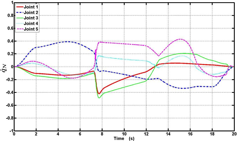
Results are shown in Fig. 3 and Fig. 5–7. Considering the manipulator has both prismatic and revolute joints, normalized joint velocity q̇N is defined as q̇iN=q̇i / ‖q̇imax‖, where q̇i and q̇imax is velocity of i th joint and maximum allowable velocity of i th joint, respectively. At the initial instant, desired torch direction and actual direction are the same. As the manipulator moves, torch direction successfully follows the desired orientation. Joint limit constraint is also guaranteed. Fig. 7 illustrates additional details related to the simulation. Time-dependent orientation constraint function Hg(q,t) value is close to the threshold at t =10.3s. Adjusting weight value w̄v1 stops further deterioration of Hg. Note that at about 14s, the value of Hg increases, and weight value w̄v1 switches sharply from near zero value to one based on Eq. (33). This accelerates Hg to move away from the lower threshold. It can be seen from Fig. 7(d) that the related virtual velocity q̇v1 is approximately zero at that moment. Chatter in the weight value does not induce a discontinuity in both virtual and actual joint velocities and is verified by Fig. 5. The same situation occurs for w̄2 at t =9.8 s. These examples verify the conclusion that discontinuity in weight setting criterion in Eq. (19) does not induce a discontinuity in the joint velocity. During the time interval between 8 to 10s, the second joint is near the joint limit, value of w̄2 has a sharp valley, falling to 0.15, at the same time, H is near the lower threshold and the related inverse weighted factor value is small. However, the system has two degrees of redundant freedom. No singularity occurs and both constraints are guaranteed. As seen from Fig. 7(f), tracking error is less than 5 × 10⁻² mm.

Trajectories of normalized joint velocities under the GWLN method.

Joint trajectories under the GWLN method, with dash lines denoting joint limits
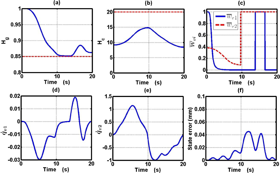
End-effector tracks the intersection line of pipes under GWLN method. (a) Orientation constraint function value Hg. (b) Joint limits compact constraint function value Hc. (c) Inverse weighted factor w̄v1 and w̄v2. (d) Virtual joint 1 velocity profile. (e) Virtual joint 2 velocity profile. (f) Norm of tracking error.
Normalized joint velocity profiles using MVN scheme
5.1.2 MVN scheme
For comparison, the MVN scheme proposed in [17] is applied to the five-link welding manipulator. MVN scheme treats constraints as dynamic changing equalities and converts the inverse kinematic problem to a dynamic-system-based QP problem Then a LVI-based numerical algorithm is exploited to solve the QP problem Thus it can be applied to the case with time-dependent constraint The welding control problem is reformulated as a QP problem as follows:
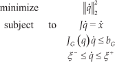
where
Fig 9 and Fig 10 show that the MVN scheme guarantees orientation constraint and keeps joints away from joint limits Position errors were less than 1×10⁻¹ mm which is larger in comparison to the result obtained using the GWLN method However this can be improved by setting a stricter stop iteration condition for the linear variational inequality-based numerical algorithm at the cost of more computations According to simulation results MVN scheme is comparatively still computationally intensive Table 2 compared simulation time for MVN scheme with GWLN method Simulations were carried out using MATLAB software with simulation control period Δt=0 01s and the task duration ttotal =20s Based on the results it can be stated that GWLN method has an advantage over the MVN scheme The MVN scheme reformulates the constrained kinematic problem into a QP problem for which obtaining an analytical solution is difficult, Although the LVI-based iteration algorithm for the QP problem has a global exponential convergence property to some extent it still complicates the process to obtain the solution [18] The average computation time of the MVN scheme is even longer than the control period shown in Table 2 Meanwhile the GWLN method directly allows the determination of the analytic solution and is comparatively faster than the iteration algorithm Considering the calculations required the MVN scheme is more suitable for off-line calculations in industrial applications.


Joint position trajectories using MVN scheme, with dash lines denoting joint limits

End-effector tracks intersection line of pipes using MVN scheme (a) Orientation constraint function value Hg. (b). Norm of tracking error.
5.2 Experimental results
The GWLN method was applied to the ZT-010 welding manipulator with five DOFs, as shown in Fig. 4. The entire system is composed of a workstation and a manipulator. The workstation is a personal digital computer with a Pentium E5300 2.6 GHz CPU, 2 GB memory, which sends instructions to the manipulator's motion controller, Turbo PMAC2-Eth-Lite stacked with PMAC2A-PC/104 (Delta Tau Data Systems Inc.). All joints of the manipulator are driven by AC servo motors (models: GYS101D5-RC2, GYS101D5-RC2, GYS401D5-RC2, GYS751D5-RC2-B and GYS102D5-RC2) manufactured by FUJI company. Servo amplifiers are matching models from the FUJI company. Servo amplifiers operate in velocity mode. Encoders attached to the motors were used to obtain the joint position.
The objective of the experiments is similar to the simulation discussed in the previous section. The start joint position is set as q(0)= 1612.68,227.95,356.91,2.64,−1.80] T , which is different from simulation. This is because the start configuration needs to set the end-effector at the start point of the pipe-to-pipe intersection seam in actual manufacturing environments and is decided by the pipe fasteners. Experimental results are shown in Fig. 11, 12 and 13. The joints successfully keep away from the joint limits. Orientation constraint function Hg nearly breaks the threshold at 19s.

Normalized joint velocity trajectories of five-link welding manipulator in welding process

Actual joint position trajectories of five-link welding manipulator in welding process, with dash lines denoting joint limits

Trajectories in the experiment. (a) Orientation constraint function value Hg. (b) Joint limits compact constraint function value Hc. (c) Inverse weighted factor w̄v1 and w̄v2. (d) Norm of tracking error.
By setting a weight factor w̄v1 less than 9×10⁻⁵, the GWLN method keeps the manipulator from breaking the orientation constraint at the end of welding process. Tracking error is less than 1.5×10⁻¹ mm, which is 190% higher than errors in simulation part. The difference is due to the disturbance on the joint velocities, shown in Fig. 11. Disturbances or iginate from the fluctuation of the mechanical payload and tracking errors of the motor servo loop.
6. Conclusion
In this paper, the GWLN method was extended to an inverse kinematic problem with a time-dependent problem, which has not been discussed in the literature and is an important area of research in recent years. By introducing time-dependent virtual joints to represent time-dependent constraints, an intermediate kinematic control problem from the virtual joint space to the revised task space is obtained. The GWLN method was then applied to obtain a uniform control law to deal with both time-dependent and time-independent constraints. In addition, a new inverse-weighted matrix setting criterion was proposed here, which allowed the simplification of the implementation of the GWLN method in comparison to previous works reported in the literature. Simulation results, including a comparison to the MVN scheme, demonstrate the efficacy and advantages of extending the GWLN method. Experiments implemented on a five-link welding manipulator verified that it was possible to realize the proposed method and to demonstrate the efficacy of the method.
However, there are two drawbacks of the GWLN method. First, the method is unable to avoid the singularity configuration. This is because the transformation of the joint space will change the criterion for singularity-avoidance joints, which is part of the transformation. Secondly, GWLN is invalid if the matrix T is not full rank, since the relationship between the virtual joint and actual joint is not mapped one-to-one. One of the major future goals of this work is related to overcoming the drawbacks of this method.
Footnotes
7. Acknowledgements
This article is a revised and expanded version of a paper entitled “Kinematic Control for Redundant Manipulators With Time Dependent Constraints: General-Weighted Least-Norm Method” presented at Control and Decision Conference (CCDC), 2014 Chinese, Changsha, China, 31 May-2 June 2014.
This work is supported by the National Natural Science Foundation of China (61074122, 61104149, 61203299), the Zhejiang Province Natural Science Fund (LY13F030001), the Program for New Century Excellent Talents in University (NCET-11-0459) and Hangzhou City major scientific and technological innovation projects of industrial chain (20132111A04-2).