Sage Journals: Discover world-class research

Abstract

In the domain of modular robotic systems, self-configuration, self-diagnosis and self-repair are known to be highly challenging tasks. This paper presents a novel fault self-diagnosis strategy which consists of two parts: fault detection and fault message transmission. In fault detection, a bionic synchronization ‘healthy heartbeat’ method is used to guarantee the high efficiency of the exogenous detection strategy. For fault message transmission, the Dijkstra method is modified to be capable of guiding the passage of fault messages along the optimal path. In a modular robotic system, fault message transmission depends mainly on local communications between adjacent modules, so there is no need for global broadcast information. Computational simulations of one system form, M-Lattice, have demonstrated the practical effectiveness of the proposed strategy. The strategy should be applicable in modular robotic systems in general.

Keywords

Modular robotic system fault self-diagnosis M-Lattice module

1. Introduction

Experience shows that failures are unavoidable in robotic systems. Several works [1,2] have reported on fault diagnosis designs applicable to single precision robots. However, few attempts have been made to construct a self-diagnosis strategy for modular robotic systems. In a collective robotic system, the probability of failure rises exponentially with increasing system scale. As a branch of collective robotic systems, modular robotic systems suffer more from unanticipated faults. Thus the diagnosis of faults in a large-scale collective robotic system such as a mobile swarm is much more complicated computationally than for a single precision robot. Compared with the conventional mobile swarm robot, the mechanism of the modular robot is simple and the processing capacity is limited. All these factors make the design of an effective fault self-diagnosis strategy for a modular system highly challenging. In this paper, an adaptive distributed self-diagnosis strategy is presented to solve this problem. Under this strategy, a single module can execute fault detection and fault message transmission using local communication channels.

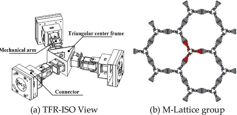
The fault self-diagnosis process is accomplished by using M-Lattice modules. M-Lattice is a type of lattice-modular robot that is designed to be capable of self-configuration, self-diagnosis and self-repair. Proper coordination of M-Lattice modules has helped assemble huge grid panels. They can be utilized to form surgery robots and solar-cell boards on solar-power satellites [3,4].

The self-diagnosis strategy consists of two parts:

1. Fault detection: In an M-Lattice system, the faults are detected exogenously by means of a ‘healthy heartbeat’ method; a healthy heartbeat signifies that the module in question has detected no endogenous fault. In order to reduce the overall communication load, each module is required to send a healthy signal periodically to its adjacent modules. If a fault-free adjacent module has not received such a signal during a certain pre-set period, it suspects that a fault has occurred and sends a fault message to the system. In a large-scale system, the detection reliability mainly depends on synchronizing communications among modules. This paper develops a synchronization method inspired by algorithms of bionic synchronization in overlay networks.

2. Fault message transmission: In an M-Lattice system, each module is capable of sending fault messages to modules that are immediately adjacent along the optimal path between the message collector and the fault detector modules. However, as the system is dynamic, the optimal path keeps changing as faults emerge. Hence, the standard Dijkstra method [5] is modified to fit the nature of the M-Lattice system. This guarantees that the message collector receives any existing fault messages with minimum delay.

1.1 Related works

The design of a diagnostic strategy is highly dependent on the implementation of the modular robotic system. Modular robots can be classified as lattice, chain and hybrid. The structure of lattice robotic systems is invariably a grid mesh, as with CHOBIE [6] and ATRON [7]. A lattice modular robot usually has more than two adjacent modules connecting with it. A chain system could be of line or tree type. As a classic chain modular robot, YaMoR [8] can crawl like a snake, rotate like a wheel or walk like an object with multiple legs. However, each YaMoR has at most two adjacent modules. Hybrid modular robots such as M-Tran [9], SuperBot [10], Roombots [11], iMobot [12] and UBot [13] have certain advantages over lattice or chain modules; for example, the number of connectors they include is sufficient to ensure high freedom redundancy. However, this makes the fault-diagnosis task more complex.

Self-diagnosis is the preliminary stage during self-repair. Several studies [14,15] have been reported in the literature on the self-repair approaches applicable to modular robots. However, few attempts have so far been made to construct a self-diagnosis strategy for modular robotic systems. Most fault detection methods have been researched in the context of mobile swarm robotic systems. In most multirobot systems, the system status including communication capacity and fault location analysis is represented as a graph [16,17]. In such graphic representations, nodes represent robots and edges represent links or communication channels between robots. This means that the fault modules can be described as insertions or deletions of edges and update edge weights accordingly. In an M-Lattice system, the weight of an edge is changeable as faulty modules emerge, which can also influence fault message transmission. Several fault detection algorithms [18,19] based on certain probabilistic fault models have proved efficiently applicable in multi-mobile robotics. The mobility of a single modular robot may be weaker than a mobile robot, but it exhibits more reliable connections with its neighbouring modules. Yim [20] presents a strategy towards the self-assembly task in a small modular robotic system. A vision-based detection method is utilized to accomplish the fault diagnosis. In huge-scale modular systems, the cost increment caused by vision cameras cannot be ignored. Not all the faults can lead to system separation, which can be detected by the vision-based method. Surprise-Based Learning (SBL) [21] is an excellent concept for the control of modular robots. SBL helps ensure robustness in the face of faults or unexpected changes in the environment by creating a predictive model of the environment on the basis of the robot's interactions with the environment. Although a single M-Lattice module may not have sufficient capability to implement SBL, a test method inspired by SBL can be used in fault detection.

This paper is organized as follows. Section 2 presents the mechanism design of the M-Lattice robot. Section 3 introduces the fault self-diagnosis strategy, including fault detection and fault message transmission. In section 4, the fault self-diagnosis strategy is tested by simulations. Finally, section 5 critiques the proposed approach and identifies opportunities for further research.

2. M-Lattice robotic system design

M-Lattice is designed to be a non-compact modular robot with one centre frame and three arms [22], as shown in Figure 1(a). The workspace of M-Lattice is a 2D plane, and each module can connect simultaneously with three neighbours - see Figure 1(b). As a distributed robotic system, each module has a controller to control its motors, communications, and monitoring of the on-board system.

Figure 1.

The M-Lattice modular robot

In order to indicate the positions of the modules, the position of the module is represented by an ordered pair of integers (r, c), where r is the row of the module's location and c the column of the module's location. The X- and Y-directions are as shown in Figure 2.

Figure 2.

The topology of the M-Lattice structure

3. A strategy for fault self-diagnosis

The modules in an M-Lattice system can be of two types: faulty and fault-free. A fault-free detector module generates a fault message whenever a fault is detected. The message will be passed through the system, and received by the host monitors placed at the system's boundary. In order to realize this diagnosis process, the fault self-diagnosis strategy should satisfy the following requirements:

Local communication is sufficient for fault detection, and global broadcast is avoided. The fault message is sent to the host monitor along the optimal path. This means the modules involved in message transmission are limited.

The number of host monitors is flexible. The absence of several host monitors only influences the optimal message transmission path; it does not cause chaos during fault detection.

The number of adjacent modules is limited. If one module has a fault, there will be several modules which can detect the fault simultaneously. This improves system reliability by increasing system redundancy.

3.1 Fault detection using a method analogous to bionic synchronization

Traditional precision robots use an endogenous fault detection method, that is, the robot tests its own working status. If there is a fault, an alarm signal is sent out. In small robot groups, such as pipeline-industry robots and robotic soccer teams, a monitor or task signal tower can be used to manage several robots and check whether any of them is faulty at a given moment. However, such an approach can lead to serious scalability problems when the system scale is large. Firstly, the processing capacity of a single module's on-board system is limited, so the module can have difficulty in detecting each and every fault as it occurs. Further, the number of system monitors increases as the scale of the robotic system becomes larger. This adds to the system's cost. If one of the monitors has a fault, all the modules being managed by it lose their fault detection abilities. This could be fatal to the system. We solve this problem by involving an exogenous fault detection method.

In our work, a ‘healthy heartbeat’ method is used as the solution. As the processing capacity of any single module is limited, it is inefficient to exchange health signals frequently. A convenient solution for this problem is to use a cycle timer that reports on the single module by periodically sending (or otherwise) a healthy heartbeat to its own neighbours. As shown in Figure 3, if one neighbour has received a heartbeat in a certain time period, the sender is considered to be healthy or fault-free. Otherwise, it is suspected that the module is unable to function due to some faults.

Figure 3.

An illustration of the healthy heartbeat method

In order to reduce the communication load, the healthy signal is binary and does not contain the status information. Although lots of factors can cause a fault in a module, it is possible to classify the faults into two types: detectable fault and undetectable fault. For detectable faults, such as actuator failure or sensor error, a single module can shut down the healthy heartbeat's sending, utilizing a finite-state machine. For undetectable faults, such as severe damage caused by a high-energy external strike or communication channel failure, where either the module is totally damaged or some communication channels are blocked, its fault-free neighbours cannot receive a healthy heartbeat. Thus, the healthy heartbeat method can handle all the fault cases in a modular robotic system.

This method is easily understood and implemented. However, in a large-scale system, it is difficult to guarantee clock cycle consistency. Although the M-Lattice module is homogeneous and the on-board oscillators are of the same type, there can be many tiny errors in the reference clocks. The accumulation of such errors over a long time can change the modules' cycle periods. Modules with shorter cycle periods cannot receive healthy signals from those with longer cycle periods, so a module that is actually fault-free gets diagnosed as a faulty module. In order to solve this problem, a bionic-type method is used to synchronize the healthy signal timer. The method is inspired by synchronous behaviours observed in nature, such as in large groups of tropical fireflies [23]. Christensen and Grady [24] use this method in swarms of robots by synchronizing the flashing cycles of LEDs placed on mobile robots. In this work, as each M-Lattice module has at most three adjacent modules, the influence of adjacent modules is limited. There is no non-synchronized error miscount and there are none of the problems of limited sensory range mentioned by Christensen and Grady.

In our work, a healthy signal timer is considered a cycle changeable oscillator and a healthy heartbeat as a signal transmitted from one module to its neighbour. The continuous model [25] can be modelled in a distributed fashion as follows:

x_{i} (n + 1) = x_{i} (n) + \frac{1}{T} + ε a_{i} (n) h (x_{i} (n))

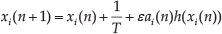
where x_i(n) is the current counter value of oscillator i, T is the number of pre-set upper-bound clock cycles, a_i(n) is the number of healthy signals received by oscillator i, and ε is a factor signifying the influence strength between adjacent oscillators. The influence function is chosen as follows:

h (x_{i} (n)) = x_{i} (n)

When x_i(n) reaches a pre-set upper bound, the module sends a healthy heartbeat to its neighbours. If a module receives a healthy signal within the time it takes to send out healthy signals twice to its neighbour, the adjacent module is deemed to be fault-free.

A synchronization example of the M-Lattice system is shown in Figure 4. The system consists of 25 M-Lattice modules. None of them is faulty. At the beginning of a synchronization exercise, the counters are set randomly between 0 and 1. The pre-set upper bound is T = 25. As shown in Figure 4(a), one module is chosen as the reference module. During the synchronization process, each module's value in each round is compared with that of the reference module. The error distribution shows the synchronization condition of the system. In the test, five modules were chosen stochastically. The synchronization processes are shown in Figure 4(b). Note that, even after 11 cycles (275 steps), all modules were working under the same clock cycle.

Figure 4.

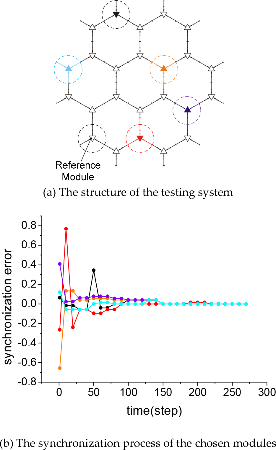
An example of synchronization with 25 modules

Further simulations were conducted to test the feasibility of the synchronization method. Firstly, the synchronization performance was tested with different influence strength factors in a system with 400 fault-free modules. As shown in Figure 5(a), certain excessive strength factors can prolong the synchronization process., because when the factor value is low the impact of its neighbours is limited and the adjacent modules need more time to stay synchronous. On the other hand, when the factor value is high, a big increment nudges the counter beyond the pre-set upper bound frequently. This oscillation makes it difficult for the system to remain in synchronicity. In the following tests, the influence strength factor, ε, is set as equal to 0.4.

Figure 5.

Synchronization simulation results

Next, faulty modules were included in a system consisting of 400 modules. The upper limit for the number of faulty modules was set at 1% of the system scale. The faulty modules were located randomly. As shown in Figure 5(b), such a synchronization process requires more time as the fault scale increases. This is because the existence of faulty modules decreases the number of fault-provoking sources around fault-free modules. The influence of small fault scale is limited since one fault-free module has just three adjacent modules and the number of faulty adjacent modules is no more than two. The distribution of the fault modules is considered as the main reason for the oscillation of synchronization time cost. Thus, the synchronization method is tolerant of faulty modules – a feature confirming the practical applicability of the fault detection strategy.

3.2 Fault message transmission

After a faulty module has been detected, the detector module generates a fault message containing the location information of the faulty module. Using local communications, the fault message can be transmitted through adjacent fault-free modules and received by the host monitors (the message collectors). The content of the fault message is as follows:

TYPE

LENGTH

SENDER

POSITION

CRC

where

TYPE means this message is a fault message;

LENGTH is the length of the message;

SENDER means the ID of the fault detector module;

POSITION contains the position information of the fault module;

CRC means the CRC check code.

As for the path-planning issue, the breadth-first gradient method is attractive in the context of an M-Lattice module. In a decentralized robotic system, we need an efficient method to represent the gradient of each module's location. The method used should recognize the limited processing capacities of individual modules, be distributed, and be adaptive to unpredictable system conditions.

The D^* algorithm [26] and the D^* Lite method [27] show good performance in the mobile robot's path-planning task. The distance-refreshing rules are heuristic for our transmission path planning. But these methods have an efficiency problem – only if the path of the mobile robot is blocked by obstacles will the path be recalculated. In our case, the transmission path is optimized in a distributed manner with high efficiency. In modular robotic systems, most heuristic algorithms are developed to solve the self-reconfiguration task. In distributed algorithms, the virtual gravity force method [28] and digital hormone method [29] have shown good performance in self-reconfiguration. But in the self-diagnosis task they suffer from the dynamic distribution of the message collectors and the efficiency problem.

Inspired by the Dijkstra method, a classical shortest path-planning method, we introduce improvements to solve the problem. This section will start with a description of the M-Lattice system topology. Next, the Dijkstra method will be explained on the basis of the structure's topology. The Dijkstra value of a module shows the distance between the positions of the module and the collector. It can be recalculated in a distributed manner. A greedy method guarantees fault message transmission along the optimal path.

3.2.1 System topology description

Having connected with each other, the M-Lattice modules form a robotic network. The network can be represented as an undirected, weighted graph G=(V, E, w), where V is a set of modular robots, E is a set of edges representing how the modules are connected, and w is a weight function. An edge (m₁, m₂) is an unordered pair of modules, m₁ and m₂. m₁ and m₂ are adjacent. In the classic graph algorithm, a path between two nodes, u and v, is a finite sequence, p = {u = v₀, v₁, v₂…v_k= v}, for each 0≤i<k, (v_i,v_i+1)∈E. The weight of the path is

w e i g h t (p) = \sum_{i = 0}^{k} w e i g h t (v_{i}, v_{i + 1})

The shortest path is the path whose weight is the smallest of all paths possible between u and v in G. The M-Lattice system is designed to be a distributed robotic system, in which there is no global message; only local communications are used. So, for a single module, u, the path between it and the target module, v, is a finite sequence, p = {u, v₀= v₁,v₂,v₃…v_k= v}, for each 0≤i<k, (v_i,v_i+1)∈ E,, and v₀ is the neighbour of u. The weight of the path is

w e i g h t (p) = w e i g h t (u, v_{0}) + \sum_{i = 0}^{k} w e i g h t (v_{i}, v_{i + 1})

As the weights between module u and its three neighbours are equivalent, the shortest path must contain the adjacent module with the shortest weight between itself and the target module, v.

3.2.2 The modified Dijkstra method

Based on the topological structure of the M-Lattice system, a Dijkstra method is used to improve the efficiency of fault message transmission. In the method, the minimum number of modules located between the current and the target modules is the Dijkstra distance, D. Each single module can hold and refresh its Dijkstra distance. The message collector is considered to be the target module, with D = 0 and D = 1 for the directly adjacent modules. As shown in Figure 6, the Dijkstra distance increases as there are more modules on the shortest path. During a fault message transmission process, each single module involved sends a fault message to its valid adjacent modules, which have the shortest Dijkstra distance.

Figure 6.

Some illustrations of Dijkstra distance

A single module can get its Dijkstra distance during self-configuration. If a change occurs in of its connection status, it will update its Dijkstra distance. The updating rules are as follows:

If one of its neighbours changes its Dijkstra distance, the module will update its own Dijkstra distance.

If there is no module on the adjacent position or a fault is suspected in the adjacent module, the Dijkstra distance of the particular neighbour's position is taken to be infinite, coded as INTMAX.

After receiving the Dijkstra distance values from all the fault-free adjacent modules, the smallest Dijkstra distance is marked as Df and the current Dijkstra distance is changed to Df + 1.

In an M-Lattice system, each message management routine operates in a distributed manner. A message management routine is run as a succession of ‘awaken-think-transmit’ cycles. In each cycle, the routine is woken up when it receives messages from adjacent modules, reads the Dijkstra distance values from all the fault-free adjacent modules, processes the values, and sends messages to the adjacent modules whose Dijkstra distance values equal the minimum. In a modular system, both the updating of Dijkstra distance and the message transmission need to occupy the local communication channel built on the connecting modules. In order to avoid the communication collision, Dijkstra distance updating is set with a higher priority. The fault message sender needs to wait until the receiver finishes the updating task. This priority distribution does decrease the transmission efficiency, but this can prevent the fault messages being transmitted to the fault modules.

In order to avoid message overload during operation, a generalized distance function is used to modify the Dijkstra method. In the following sections, the acquisition of the Dijkstra distance from the generalized distance function will be labelled as the Modified Dijkstra distance (MD distance), and the previous Dijkstra distance is labelled as the Standard Dijkstra distance (SD distance). The generalized distance function is then defined as follows:

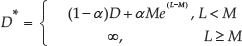
D^{*} = {\begin{matrix} (1 - α) D + α M e^{^{(L - M)}}, L < M \\ \infty, L \geq M \end{matrix}

(1)

where D is the SD distance of the current module, M is the maximum communication load of a single module, L is the current communication load of the module, α is the function coefficient set as 0.02 in subsequent tests, and D^* is the MD distance of the current module. If and when a module has already received too many fault messages, its MD distance increases, and a new fault message will not be sent to it. It is evident from Equation (1) that, when the SD distance is small, the corresponding MD distance depends mainly on the current communication load because the SD distance is independent of the communication load. This feature substantially hinders message blocking by a single module that is near the message collector with a small SD distance.

4. Simulations of fault self-diagnosis

The fault self-diagnosis process was simulated on MATLAB, running on a desktop with a CPU Pentium E5200 Dual-Core, RAM 2 GB. The system was initialized under the presentation of an undirected weighted graph, G=(V, E, w). As mentioned above, w was the weight of the connection between adjacent modules. In the experiments, it equalled the Dijkstra distance increment between connecting modules. The system form was set as a rectangle. The message collectors were set in the required positions, and the modules could refresh their Dijkstra distance values automatically.

The flow diagram of fault self-diagnosis is shown in Figure 7. Firstly, the system scale, the positions of message collectors and the message load capacity of single module are initialized. After the simulation has started, certain randomly chosen modules are set as faulty modules. If a module detects that one of its neighbouring modules is faulty, it sends a fault message containing the position information of the fault module to its neighbour with the minimum Dijkstra distance. The number of fault messages generated by fault-free modules is compared with the number of fault messages received by message collectors. The path of each fault message transmission is saved by the simulator. If no messages are passing through the system, the simulation round is considered to be complete.

Figure 7.

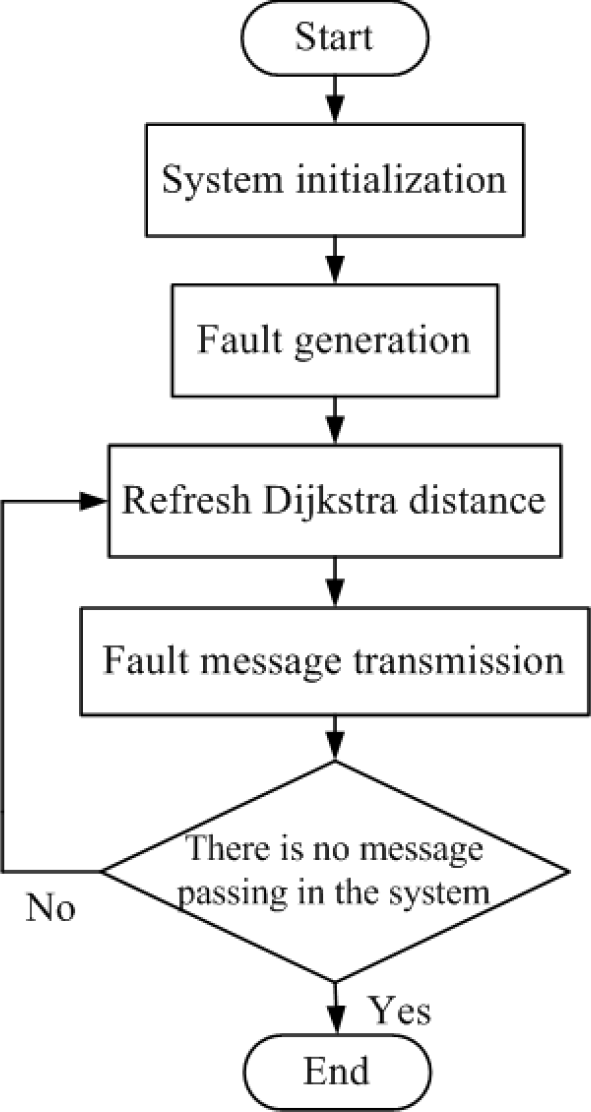
Flow diagram of fault diagnosis

4.1 Scalability and improvement by multi message collectors

In order to test the scalability of the diagnosis strategy, the system scale was set between 50times50 and 200times200. It was assumed that there was one message collector at position (0,0), that the number of fault modules was 1% of the system scale, and that the message capacity of a single module was infinite. The simulations were repeated 30 times for each system scale.

The results of the simulations are shown in Figure 8. The vertices of the triangles in the 2D plane are the positions of the faulty modules, which are chosen randomly in the simulations, and the colour bar indicates the path length of message transmission. In order to find the relationships between path length and fault position, all faulty modules belonging to different test rounds are plotted in a single figure for each system scale. If one module appears in several test rounds, the average length value is used. For modules which are never chosen as fault modules, the length values of these positions are estimated by the Delaunay triangulation interpolation method. It is thus found that, compared with the results obtained at different system scales, the length of the message transmission path when the scale of fault modules is small depends mainly on the distance between the faulty modules and the message collector. This establishes the scalability of the system.

Figure 8.

Fault diagnosis with different system scales

It is unreliable to place only one message collector in a huge system. Multi-message collectors can increase the robustness of system monitoring as well as the message transmission efficiency. In this test, the system scale was set at 100times100, the fault number at 1% of system scale, and the number of message collectors in the range two to four. The message collectors were placed symmetrically around the boundary of the system with a view to decreasing mutual influences.

As shown in Figure 9, the maximum path length becomes shorter with more message collectors. As the Dijkstra distance of the message collector is 0, adding more message collectors will decrease the average system Dijkstra distance. In addition, since fault messages can be sent to the nearest message collector, parallel message processing can increase the efficiency of diagnosis.

Figure 9.

Diagnosing faults using multi-message collectors

4.2 Diagnosis under big scales of fault modules

A larger scale of faulty modules lowers the fault detection rate. As shown in Figure 10(a), the system scale was 50times50, and the number of fault modules varied between 10% and 60% of the system scale. Although adding more message collectors can increase the fault-tolerant redundancy, the detection rate is extremely low when the fault scale exceeds 30%. This is because when the fault scale becomes larger, the probability of the transmission path being cut off becomes higher. Hence, the system becomes incapable of detecting faulty modules surrounded by other faulty modules. Although not all the fault modules can be detected directly through the fault messages, the system can still estimate the scale of faulty modules. As shown in Figure 10(b), if we can detect that several faulty modules are connecting together and forming a closed region, the modules within this region can be considered faulty, so the fault scale can be estimated.

Figure 10.

Diagnosis under big scales of faulty modules

4.3 Influence of message load capacity

During actual use of the M-Lattice system, the message load capacity of a single module cannot be infinite. As mentioned above, the message load can change the module's Dijkstra distance and then change the message transmission path. In this test, the system scale was set at 50times50, and the number of fault modules at between 5% and 15% of the system scale. The number of message collectors was set separately as one and four. The message load capacity was changed from one to 10 messages. In each test round, the Dijkstra distance was calculated under the Standard Dijkstra (SD) method and the Modified Dijkstra (MD) method separately. The continuous message transmission was decomposed into a sequence of discrete steps. In each step, a single module chose one fault-free module, which had the smallest Dijkstra distance, and sent fault messages to it. If message overload happened, the rest of the messages were sent in the next step.

The simulation results are shown in Figure 11. Firstly, the improvement of diagnosis efficiency caused by the message load capacity increment is not infinite. As there are spatial differences among faulty modules, there always exist temporal differences associated with fault message transmission. But the high system cost caused by a single module's load capacity increment cannot be ignored at the same time. Secondly, with the same fault scale and message load capacity, the MD method performs better than the SD method. This is because the current message load is considered to be of the feed-forward type while calculating the Dijkstra distance. This decreases the probability of message overload, and proves the practical validity of the MD method. Finally, it is found that the increment of message collectors only affects the diagnosis efficiency, which has been proven previously, and does not change the relationship between message load capacity and fault scale.

Figure 11.

Diagnosis with changeable message load capacity

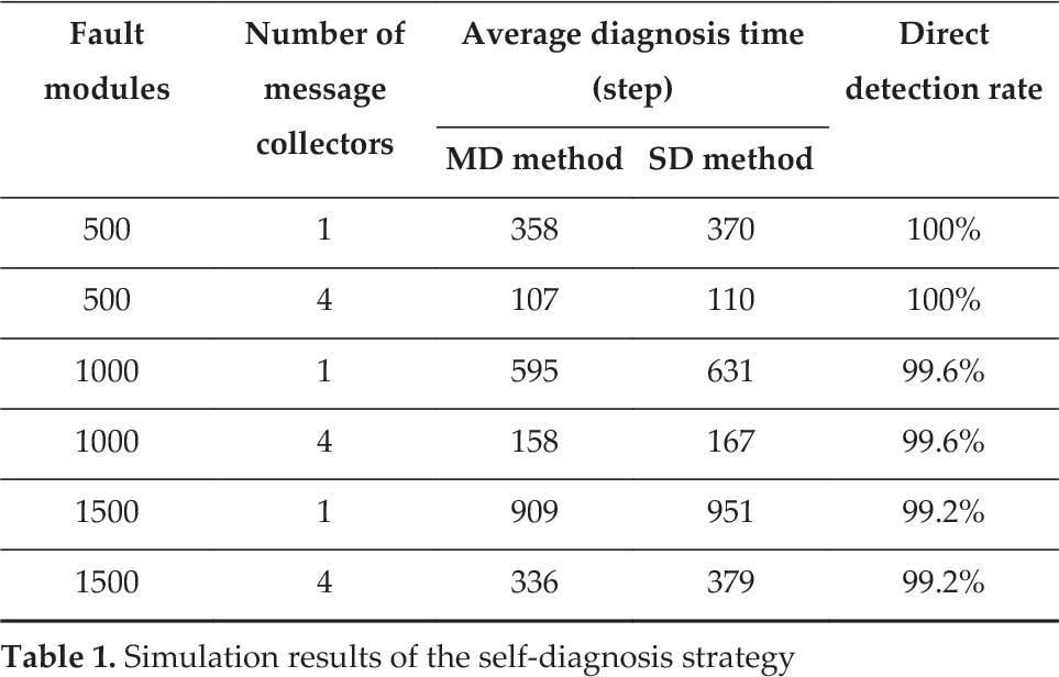
Finally, the self-diagnosis strategy was tested in a huge M-Lattice system. In this test, the system scale was set at 100times100. The number of fault modules was set separately as 5%, 10% and 15% of the system scale. The number of message collectors was set separately as one and four. They were placed symmetrically around the boundary of the system. The message load capacity was six messages. The MD method and SD method were chosen to calculate the Dijkstra distance separately. The faulty modules were located randomly. In each fault scale, the simulations were repeated 30 times. The simulation results are shown in Table 1. The MD method shows better performance than the SD method, especially in a large-fault-scale condition. From the results, it can be seen that the self-diagnosis strategy has a reasonable success rate in a huge-scale system. Reliability is guaranteed with different numbers of message collectors.

Table 1.

Simulation results of the self-diagnosis strategy

Fault modules	Number of message collectors	Average diagnosis time (step)		Direct detection rate
Fault modules	Number of message collectors	MD method	SD method	Direct detection rate
500	1	358	370	100%
500	4	107	110	100%
1000	1	595	631	99.6%
1000	4	158	167	99.6%
1500	1	909	951	99.2%
1500	4	336	379	99.2%

From the simulation results, it can be concluded that the diagnosis strategy is reliably scalable under small scales of fault modules. Multi-message collectors can increase the robustness and efficiency of system detection. The scale of faulty modules can be estimated by analysing the fault messages received when the fault scale is large. By improving the standard Dijkstra method, one can improve the robustness of the system in the presence of increasing fault scale. This represents a balance between the cost control and system diagnosis property. In the future, we want to improve the diagnosis strategy in order to guarantee the detection correctness in the synchronization process. How to execute diagnosis strategy in self-configuration and self-repair will be a key issue in further research.

5. Conclusions

This paper has introduced a novel fault self-diagnosis strategy for modular robotic systems. The validity and high efficiency of the strategy for M-Lattice robotic systems have been demonstrated. The strategy has the advantages that local communication is sufficient for fault diagnosis and global broadcast is avoided. The fault message is sent to the message collector along the optimal path, which means the modules involved in message transmission are limited. Under the ‘healthy heartbeat’ method, a faulty module can be detected by several adjacent fault-free modules simultaneously. This increases the system's reliability redundancy. A method analogous to the bionic synchronization method is used to guarantee the high efficiency of the fault detection strategy. Further, the improvement in comparison to the standard Dijkstra method makes the method more suitable for message transmission through the modular robotic system. Results from simulations have shown that the fault self-diagnosis strategy is efficient and systematic and is generally applicable in the domain of scalable modular robotic systems.

Footnotes

6. Acknowledgements

This work was partially supported by the National Natural Science Foundation of China (under Grant No. U1401240, 61473192) and the Medical Cross Fund Project of SJTU (Grant No.YG2012MS53).

References

Yang

(2002) Fault-tolerant gaits of quadruped robots for locked joint failures. IEEE Transactions on Systems, Man and Cybernetics Part C: Applications and Reviews. Vol. 32, no. 4, pp. 507–516.

Van

Kang

Suh

Shin

(2013) A Robust Fault Diagnosis and Accommodation Scheme for Robot Manipulators. International Journal of Control, Automation and Systems. Vol.11, no.2, pp. 377–388.

Rouge

(2007) Space-based Solar Power As an Opportunity for Strategic Security. Phase 0 Architecture Feasibility Study, Report to the Director, National Security Space Office.

Mankins

Kaya

Vasile

(2012) SPS-ALPHA: The First Practical Solar Power Satellite via Arbitrarily Large Phased Array. Annual International Energy Conversion Engineering Conference (IECEC). 2012, July 30–Aug. 1; Atlanta, USA. AIAA. pp. 1–13.

Dijkstra

(1959) A note to two problems in connection with graphs. Numerische Mathematik. Vol. 1, no. 2, pp. 269–271.

Suzuki

(2008) Reconfigurable Modular Robot Adaptively Transforming a Mechanical Structure. J. Robot. So. Vol. 26, no. 1, pp. 74–81.

Østergaard

(2006) Design of the ATRON lattice-based self-reconfigurable robot. Autonomous Robots. Vol. 21, no. 2, pp. 165–183.

Moeckel

Jaquier

Drapel

(2006) Exploring adaptive locomotion with YaMoR, a novel autonomous modular robot with Bluetooth interface. Industrial Robot: An International Journal. Vol. 33, no. 4, pp. 285–290.

Murata

Yoshida

Kamimura

(2002) M-TRAN: Self-Reconfigurable Modular Robotic System. IEEE/ASME Transactions on Mechatronics. Vol. 7, no. 4, pp. 431–441.

10.

Salemi

Moll

Shen

(2006) SUPERBOT: A Deployable, Multi-functional, and Modular Self-Reconfigurable Robotic System. IEEE/RSJ International Conference on Intelligent Robots and Systems (IROS). 2006, Oct. 9-15; Beijing, China. IEEE. pp. 3636–3641.

11.

Sproewitz

Laprade

Bonardi

(2010) Roombots – Towards Decentralized Reconfiguration with Self-Reconfiguring Modular Robotic Metamodules. IEEE/RSJ International Conference on Intelligent Robots and Systems (IROS). 2010, Oct. 18-22; Taipei, Taiwan. IEEE. pp. 1126–1132.

12.

Ryland

Cheng

(2010) Design of iMobot, an Intelligent Reconfigurable Mobile Robot with Novel Locomotion. IEEE International Conference on Robotics and Automation (ICRA). 2010, May 3-7; Anchorage, USA. IEEE. pp. 60–65.

13.

Zhao

Cui

Zhu

Tang

(2012) UBot: A new reconfigurable modular robotic system with multimode locomotion ability. Industrial Robot: An International Journal. Vol. 39, no. 2, pp. 178–190.

14.

Cicerone

Stefano

Frigioni

Nanni

(2003) A fully dynamic algorithm for distributed shortest paths. Theoretical Computer Science. Vol. 297, no. 1, pp. 83–102.

15.

Rus

Vona

(2000) A basis for self-reconfiguring robots using crystal modules. IEEE/RSJ International Conference on Intelligent Robots and Systems (IROS). 2000, Oct. 31–Nov. 5; Takamatsu, Japan. IEEE. pp. 2194–2202.

16.

Tomita

Murata

Kurokawa

Yoshida

Kokaji

(1999) Self-Assembly and Self-Repair Method for a Distributed Mechanical System. IEEE Transactions on robotics and automation. Vol. 15, no. 6, pp. 1035–1045.

17.

Mourad

Nayak

(2012) Comparison-Based System-Level Fault Diagnosis: A Neural Network Approach. IEEE Transactions on Parallel and Distributed Systems. Vol. 23, no. 6, pp. 1047–1059.

18.

Garcia

Schultz

Stoy

(2009) On the Efficiency of Local and Global Communication in Modular Robots. IEEE/RSJ International Conference on Intelligent Robots and Systems (IROS). 2009, Oct. 11-15; St. Louis, MO. IEEE. pp. 1502–1508.

19.

Martin

Emami

(2013) A fault-tolerant approach to robot teams. Robotics and Autonomous Systems. Vol. 61, no. 12, pp. 1360–1378.

20.

Yim

Shirmohammadi

Sastra

(2007) Towards robotic self-reassembly after explosion. IEEE/RSJ International Conference on Intelligent Robots and Systems (IROS). 2007, Oct. 29–Nov. 2; San Diego, USA. IEEE. pp. 2767–2772.

21.

Ranasinghe

Shen

(2011) Autonomous Adaptation to Simultaneous Unexpected Changes in Modular Robots. IEEE/RSJ International Conference on Intelligent Robots and Systems (IROS). 2011, Sep. 25-30; San Francisco, CA. IEEE.

22.

Guan

Yan

Jiang

(2010) A Novel Design for the Self-reconfigurable Robot Module and Connection Mechanism. International Conference on Intelligent Robotics and Applications (ICIRA). 2010, Nov. 10-12; Shanghai, China. IEEE. pp. 400–408.

23.

Buck

(1988) Synchronous rhythmic flashing of fireflies II. Quart. Rev. Biol. Vol. 63, no. 3, pp. 265–289.

24.

Christensen

O'Grady

Dorigo

(2009) From Fireflies to Fault-Tolerant Swarms of Robots. IEEE Transactions on Evolutionary Computation. Vol. 13, no. 4, pp. 754–766.

25.

Izhikevich

(1999) Weakly pulse-coupled oscillators, FM interactions, synchronization, and oscillatory associative memory. IEEE Transactions on Neural Networks. Vol. 10, no. 3, pp. 508–526.

26.

Stentz

(1994) Optimal and efficient path planning for partially-known environments. IEEE International Conference on Robotics and Automation (ICRA). 1994, May 8-13; San Diego, USA. IEEE. pp. 3310–3317.

27.

Koenig

Likhachev

(2005) Fast replanning for navigation in unknown terrain. IEEE Transactions on Robotics. Vol. 21, no. 3, pp. 354–363.

28.

Christensen

Østergaard

Lund

(2008) Metamodule Control for the ATRON Self-Reconfigurable Robotic System. International Conference on Intelligent Automation Systems (IAS). 2008, March 7-9; Amsterdam, Netherlands. pp. 685–692.

29.

Shen

Salemi

Will

(2002) Hormone-inspired adaptive communication and distributed control for CONRO self-reconfigurable robots. IEEE Transactions on Robotics and Automation. Vol. 18, no. 5, pp. 700–712.

Fault Self-Diagnosis for Modular Robotic Systems Using M-Lattice Modules

Abstract

Keywords

1. Introduction

1.1 Related works

2. M-Lattice robotic system design

3. A strategy for fault self-diagnosis

3.1 Fault detection using a method analogous to bionic synchronization

3.2 Fault message transmission

3.2.1 System topology description

3.2.2 The modified Dijkstra method

4. Simulations of fault self-diagnosis

4.1 Scalability and improvement by multi message collectors

4.2 Diagnosis under big scales of fault modules

4.3 Influence of message load capacity

5. Conclusions

Footnotes

6. Acknowledgements

References