Sage Journals: Discover world-class research

Abstract

Map generation by a robot in a cluttered and noisy environment is an important problem in autonomous robot navigation. This paper presents algorithms and a framework to generate 2D line maps from laser range sensor data using clustering in spatial (Euclidean) and Hough domains in noisy environments. The contributions of the paper are: (1) it shows the applicability of density-based clustering methods and mathematical morphological techniques generally used in image processing for noise removal from laser range sensor data; (2) it presents a new algorithm to generate straight-line maps by applying clustering in the spatial domain; (3) it presents a new algorithm for robot mapping using clustering in a Hough domain; and (4) it presents a new framework to load, delete, install or update appropriate kernels in the robot remotely from the server. The framework provides a means to select the most appropriate kernel and fine-tune its parameters remotely from the server based on online feedback, which proves to be very efficient in dynamic environments with noisy conditions. The accuracy and performance of the techniques presented in this paper are discussed with conventional line segment-based EKF-SLAM and the results are compared.

Keywords

Robot mapping clustering noise reduction Hough transform

1. Introduction

Autonomous navigation by a mobile robot in an unknown environment is an important problem in mobile robotics. The robot mainly perceives the outer world by utilizing measurement sensors attached to it. These sensors (typically laser range finders, ultrasonic sensors, cameras and 3D sensors) give an estimate of the robot's position in the environment and incrementally build the map of the environment. This problem is often referred to as ‘simultaneous localization and mapping’ (SLAM), in which a robot simultaneously localizes its position in the environment and builds a map of it. Hence, it becomes important for the robot to have an accurate map. While sensors such as wheel encoders measure the relative robot displacement, external sensor data can be used to correlate subsequent robot positions to get the relative pose or estimate, improving upon the odometry data. However, in reality, sensors are prone to errors and generate noise in the data. This noise then accumulates as error over time and gives the wrong estimate or else the wrong map. The environments in which the robot navigates are mostly dynamic, which adds to the complexity of the mapping. The main task of the robot is to incrementally build the map of the workspace as it discovers the environment, and to avoid obstacles, in order to reach its final goal. Various approaches to solving this problem have been discussed by researchers. An earliest attempt to solve the SLAM problem was proposed in work given in [40], in which uncertainty models were introduced to solve the localization and mapping simultaneously. The trajectories and positions of landmarks in the environment are estimated without any need for prior knowledge of the location of the landmark. To get a complete perception of the region, the scan data from the sensors must be matched and fused in order to get a desirable map of the region [19]. In [45], various methods for solving SLAM are discussed in detail, including the extended Kalman filter SLAM (EKF-SLAM) as well as particle filters. Many have looked to solve SLAM using visual sensors, like cameras [4]. Recently, 3D sensors, like MS-Kinect, have also been employed to map surroundings [37].

There are two common techniques used in mobile robotics for mapping: (1) point-based matching, and (2) feature-based matching. In the first technique, measured data points are directly used for mapping, such as in [20] where they utilize range data to localize in a polygonal environment. Using an iterative least squares minimization technique, they proposed a matching algorithm between point images and target models in an a priori map. A study by [16] proposed a similar self-localization approach, but not necessarily in a polygonal environment. Their algorithm iteratively improves the alignment between two scans by minimizing the distance between them. A major drawback of using point-based matching is that it requires a large amount of memory to handle and the storage grows disproportionately for large environments, which in turn reduces performance. The other technique for working with scan data involves utilizing the raw measurement points into geometric features by transforming the raw scans into meaningful features. These features can then be used for matching and scan corrections. In comparison to point-based matching, feature-based matching techniques require less memory, are more efficient and provide more information about the environment. In addition, the extracted features, such as corners and line segments, can be subsequently used as building blocks for localization or mapping. Large data can be scaled down to simple geometric features, even for large environments. Because of these reasons, feature-based matching has been extensively researched and employed into SLAM. Feature extraction, feature tracking and efficient mapping algorithms work with much less data and are more stable, specially when dealing with noise. In most scenarios in which mobile robots work (both indoors and outdoors), planar surfaces are common and they are typically modelled by line segments. Line segments are the simplest geometric primitives used to describe structural environments. The work in [48] presents an extensive survey and summary of line feature extraction algorithms from range sensors for indoor mapping, including split and merge [17], incremental [33], a Hough transform [41, 15, 25], line regression [27], RANSAC [31] and an expectation-maximization algorithm [13, 43].

This paper only focuses on the mapping problem, using laser range finder (LRF) data in noisy environments. The present work is a larger extension of our previous work [2, 3], in which we proposed mapping using clustering techniques. The authors have extended the work by proposing new noise removal algorithms and mapping techniques in this paper. For accurate map building, we first tackle the problem of removing noise from the LRF data. The noise results in the generation of inaccurate maps and it must be removed. Noise reduction in SLAM has been discussed in [6, 36, 18]. This paper propose using density-based clustering algorithms and mathematical morphological kernels like dilation and erosion to remove noise. These techniques have mainly been used in processing images - our results show that they are also effective for noise removal from LRF data. For noise removal using mathematical morphological techniques, this paper provides various kernels which can be selected according to the nature of the noise present in the LRF data. We also propose a new algorithm for extracting line segments using clustering in a Hough domain. This algorithm can detect line segments effectively in cluttered narrow environments with noisy data.

The algorithms proposed in this paper are mainly clustering-based. Clustering is the main technique used in exploratory data mining, and is a common technique for statistical data analysis used in many fields, including machine learning, pattern recognition, image analysis, information retrieval and bioinformatics [1]. Clustering has been applied to SLAM as well. In [28], the authors proposed a nested dissection algorithm which leads to a cluster tree for a multilevel sub-map-based SLAM. In [17], a combined Kalman filtering and fuzzy clustering algorithm is proposed. The work in [8] proposed a convolution-based clustering algorithm and a Hough transform-based line tracker using a laser scanner. In [49], a technique for online segment-based map building in an unknown indoor environment from sonar sensor observations is proposed. An enhanced adaptive fuzzy clustering algorithm (EAFC) along with noise clustering (NC) is proposed to extract and classify the line segments in order to construct a complete map for an unknown environment. Recent works like [9] have proposed a method called ‘distance-based convolution clustering’ (DCC), in which the robot's scanned points are grouped into clusters using a convolution operation. They also proposed a new algorithm to detect lines by appending a cluster of points using a combined Hough transform and line-tracking algorithms. Another work by [32] presented clustering methods to convert data points into point clusters and line segments. They used a rank order clustering (ROC) technique where prior information on a number of clusters is not required. A similarity index matrix (SIM) using fuzzy membership is used to extract and merge suitable line segments. Meanwhile, in [9], a ‘reduced Hough transform line tracker’ (REHOLT) is discussed, where voting in the accumulator space in the Hough domain is reduced by first fitting the scan points by a line tracking algorithm and then obtaining a single line using the Hough transform method. It requires tuning the parameters obtained from the line tracking algorithm prior to getting a good estimate of the position of the line. Our technique for line segment extraction does not require such prior adjustment and can detect single straight lines from the scanned data points. A random window randomized Hough transform (RWRHT) is proposed in [5] to find line segments from an image. The ‘randomized Hough transform’ (RHT) method is based on the fact that a single parameter item can be determined uniquely with a pair of edge points [14]. Such point pairs are selected randomly, the parameter point is solved from the line equation and the corresponding cell is accumulated in the accumulator space. The authors extended the RHT by clustering a variable bandwidth mean shift algorithm. Cluster modes are selected as the set of base lines. Next, projections on the edge points onto the corresponding base lines are grouped to obtain the line segments.

We also present a framework for robot map building to load, delete or fine-tune the parameters of the map building applications in the robot. This can be done by a remote user based on feedback. The framework allows temporary maps to be seen on the server, and this live update enables the user to change the parameters of the map-building applications of the robot. Thus, the framework provides flexibility for changing or tuning the software according to the nature of the noise present in the environment by the user based on feedback.

Finally, we present experimental results in both artificial and real environments and discuss maps obtained by the proposed algorithms. The proposed algorithm is compared with traditional line segment-based EKF-SLAM and the results are discussed.

2. Robot Odometry

This section describes the robot model and the LRF used for the experiments. The odometry model of the robot is derived in order to obtain the accurate position of the robot. Δx and Δy represent the displacement in the x and y directions respectively, and Δθ represents the angular displacement in the counter-clockwise direction. Figure 1(a) shows the differential drive robot (Model:Plat-F1, Japan Systems Design) used during the experiments. The sensor used for the experiment is the scanning LRF (URG-04LX) manufactured by Hokuyo Co. Ltd shown in Figure 1(b). The specifications of the laser sensor have been summarized in Table 1.

Table 1.

Laser range sensor specifications

Laser range sensor	URG-04LX
Distance range	60 mm ~ 4000 mm
Accuracy	20 ~ 1000 mm: ±25 mm
	1000 ~ 4000 mm: ±2.5%
Distance resolution	3.8 mm ((4000–60)mm / 1024)
Scan angle	240 deg
Angular resolution	1.875 deg (240 deg/128)

Figure 1.

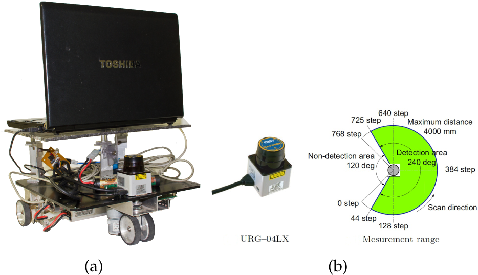
Description of the robot and sensor used for the experiments: (a) a differential drive robot (Plat-F1) with a laser sensor, and (b) Hokuyo URG-04LX specifications

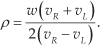
The robot coordinate frame system is defined as shown in Figure 2. The global and local coordinate system for the robot are represented by O − xy and O′ − x′y’, respectively. The diameter of the wheels is d and the tread is given by w. The midpoint of w is fixed at point O’, which is the origin of the local coordinate system O′ − x′y′ fixed on the robot. The robot moves in the direction y′ perpendicular to the direction x′ The angle θ is the angle between the y′ axis and the x axis in a counter-clockwise direction. The rotational angle of the left wheel (φ_L) and the right wheel (φ_R) is defined in the forward direction of motion. The angular rotation of the robot is given by ω. The velocities of the wheels of the robot υ_L and υ_R are expressed as:

Figure 2.

Robot coordinate frame system

υ_{R} = {\dot{ϕ}}_{R} d, υ_{L} = {\dot{ϕ}}_{L} d

(1)

Here, φ represents the differential operator with respect to time t. From Figure 2(a), considering the circular motion and the curvature radius ρ, we can define the velocity υ as:

υ = ρ ω .

(2)

On the other hand, using the tread w, υ_L and υ_R can be written as:

υ_{R} = (ρ + \frac{w}{2}) ω, ​ υ_{L} = (ρ - \frac{w}{2}) ω .

(3)

Using Equations (1), (2) and (3), the following relationships are obtained:

ω = \frac{(υ_{R} - υ_{L})}{w},

(4)

υ = \frac{(υ_{R} + υ_{L})}{2},

(5)

and:

ρ = \frac{w (υ_{R} + υ_{L})}{2 (υ_{R} - υ_{L})} .

(6)

Here, assuming υ and ω as constant values during time [t₀,t₁), integrating Equations (5) and (6) in the interval [t₀,t₁] yields the following equations:

(t_{1} - t_{0}) ω = \frac{(D_{r} (t_{1}) - D_{r} (t_{0})) - (D_{l} (t_{1}) - D_{l} (t_{0}))}{w},

(7)

(t_{1} - t_{0}) υ = \frac{(D_{r} (t_{1}) - D_{r} (t_{0})) + (D_{l} (t_{1}) - D_{l} (t_{0}))}{2},

(8)

where the displacement of the left and right wheels at time t is D_l(t) and D_r(t). From Equations (7) and (8), the robot's displacement and orientation with respect to O – xy are given by:

Δ θ = \frac{(D_{r} (t_{1}) - D_{r} (t_{0})) - (D_{l} (t_{1}) - D_{l} (t_{0}))}{w},

(9)

Δ x = \frac{(D_{r} (t_{1}) - D_{r} (t_{0})) + (D_{l} (t_{1}) - D_{l} (t_{0}))}{2} \cos θ (t_{0}),

(10)

Δ y = \frac{(D_{r} (t_{1}) - D_{r} (t_{0})) + (D_{l} (t_{1}) - D_{l} (t_{0}))}{2} \sin θ (t_{0}) .

(11)

Assuming that Δθ is sufficiently small, from Equations (9), (10) and (11), we get the displacement from time [t₀,t₁]. The sensor data at time t₀ is represented at O − xy and the sensor data at time t₁ is represented by O′ − x′y′. In the next section, these parameters (Δx, Δy, Δθ) will be used to define algorithms for map generation.

3. Clustering in the Spatial Domain

This section describes LRF data clustering in the spatial domain for robot mapping. A spatial domain represents LRF data in space (i.e., x,y coordinates for the 2D case) with the direct manipulation of the LRF data during its processing. Clustering (ex. k-means clustering) is sensitive to noise [35], which may result in inaccurate cluster formation. Therefore, it is necessary to first remove noise from the LRF data and then apply clustering. Noise removal is discussed in Section 3.2.1 and Section 3.2.2, while clustering using k - means and fuzzy- c means in the spatial domain is discussed in Section 3.3.

A robot with a LRF mounted on it moves in small steps, which are the robot's displacement in step-time $Δ s_{t_{n}} = t_{n} - t_{n - 1}$ within the two time intervals t_n−1 and t_n. From Equation (11), for the robot's movement perpendicular to the x -axis, θ = 90 degrees and displacement Δx = 0, while displacement Δy is given by:

Δ y = \frac{(D_{r} (t_{n}) - D_{r} (t_{n - 1})) + (D_{l} (t_{n}) - D_{l} (t_{n - 1}))}{2},

(12)

Once the data is read from the LRF, it is grouped into segments Sⁱ,i>0, as shown in Figure 4, using the data segmentation techniques described in Section 3.1. In each step-interval ΔS_t, the raw LRF data obtained is segmented. Later, techniques for noise removal or clustering are applied to each segment.

Figure 3.

(a) Online Mode, (b) Offline Mode, and (c) Mixed Mode. The red dots represent the centroid obtained after clustering.

Figure 4.

LRF data segmentation

We define the following three modes for map generation after the noise reduction and clustering of the raw LRF data to generate maps:

Online Mode: In Online Mode, the robot continuously applies noise reduction and clustering on the data as soon as they are available with each scan after the step-interval ΔS_t. Figure 3(a) shows the working of the robot in Online Mode. Lhe raw LRF data measured at each step-interval $Δ s_{t_{n}} = t_{n} - t_{n - 1}$ is shown in Figure 3(a)-(i). In each step-interval ΔS_t, two operations are performed. First, noise is removed by the methods discussed in Section 3.2.1 and/or Section 3.2.2. The noise removed at each ΔS_t is shown in Figure 3(a)-(ii). Later, in the same step-interval, clustering is performed, as described in Section 3.3, to obtain single or multiple clusters. This is shown in Figure 3(a)-(iii) with the red dots representing the centroids of individual clusters. Generally, any given single cluster (and hence a single centroid) obtained in each step-interval as raw LRF data in ΔS_t is small. However, multiple clusters (and hence multiple centroids) can also be obtained if the raw LRF in ΔS_t is large enough. The data which has been processed once in a step-interval $Δ s_{t_{n}}$ is marked as ‘processed’ and is not processed again in the next step-interval $Δ s_{t_{n + 1}}$ . Thus, in $Δ s_{t_{n + 1}}$ , noise removal and clustering is applied on newly obtained data and the process is repeated.

Offline Mode: In this mode, raw LRF data is accumulated until a predefined $N_{s_{\max}}$ time-steps (ΔS_t), and noise reduction and clustering is applied on the accumulated (offline) LRF data after $N_{s_{\max}} \times Δ s_{t}$ steps for a given θ. This is shown in Figure 3(b). Offline Mode is useful when step-time ΔS_t produces very little data, which is inefficient for clustering. The raw LRF data is shown in Figure 3(b)-(i) obtained at each step-interval $Δ s_{t_{n}} = t_{n} - t_{n - 1}$ . Here, $N_{s_{\max}}$ is set to ‘9’. Unlike Online Mode, two operations of noise removal and clustering are applied to the accumulated LRF data after 9 × ΔS_t step-intervals. Figure 3(b)-(i) shows the accumulated LRF data with $N_{s_{\max}}$ . Figure 3(b)-(ii) shows the results of the noise removal. Figure 3(b)-(iii) shows nine centroids obtained after the clustering of the offline data. Notice that the number of clusters of offline data may vary. For example, Figure 3(b)-(iv) shows five centroids obtained after the clustering of noise-free data shown in Figure 3(b)-(ii). However, if the robot changes it's direction (i.e., for a change in θ), noise removal and clustering are applied after n × ΔS_t, even if $n < N_{s_{\max}}$ , to eliminate data processing for the special case when θ changes during accumulation.

Mixed Mode: In Mixed Mode, some of the LRF data processing takes place in Online Mode, whereas others take place in Offline Mode. For example, noise reduction and clustering can take place in Online Mode and Offline Mode, respectively. This is shown in Figure 3(c). The LRF data is scanned at each step-interval as shown in Figure 3(c)-(i). Noise is removed after each step-interval, as shown in Figure 3(c)-(ii). However, clustering is performed on accumulated (offline) data after 3 × ΔS_t step-intervals (N_{s_max} =3). Three clusters are made offline, as shown in Figure 3(c)-(iii), whereas two clusters are shown in Figure 3(c)-(iv).

3.1 LRF Data Segmentation

Prior to extracting lines, the LRF data is pre-processed into distinct segments. The LRF scans the environment and acquires n scan points, represented as:

P_{i} = [x_{i}, y_{i}] = [r_{i} \cos φ_{i}, r_{i} \sin φ_{i}], ​ i = 1, 2, \dots, n

(13)

where r_i is the distance between the i^th scanned point with respect to the origin of the LRF, and φ_i is the angle of the i^th scan point with respect to the X_L axis of the LRF frame given by O − X_L Y_L in Figure 5.

Figure 5.

Geometry of a scanned point and a corresponding line

Initially, we adopted the standard split and merge technique [48] for segmenting the data without line extraction for its robustness and speed. In the split process, we used the adaptive breakpoint detector (ABD) method to detect any discontinuity in the data [17,10]. This can make inferences about the possible presence of discontinuities in a sequence of valid range data. In the real world, such discontinuity accounts for open doors, windows, open passages and other areas which it is important to recognize. A point distance-based segmentation (PDBS) method detects these breakpoints by finding the Euclidean distance between the two consecutive points P_i and P_i+1:

‖ P_{i + 1} - P_{i} ‖ < D_{t h}

(14)

ABD uses the distance threshold D_th via the following:

D_{t h} = r_{i} \frac{\sin (Δ ϕ_{a})}{\sin (λ - Δ ϕ_{a})} + 3 σ_{r}

(15)

where Δφ_a is the angular resolution of the LRF and σ_r is the residual variance to encompass the stochastic behaviour of the sequence of the scanned points p_i and the related noise associated with r_i. The deviation is provided by the LRF manufacturer and λ is an auxiliary parameter. The value of λ has been found to perform well when setting the value as λ = 10.

After getting the breakpoints, the clusters are split using the iterative end point fitting (IEPF) algorithm [42] and segments Sⁱ are obtained. IEPF is a recursive algorithm for line extraction and for finding clusters. The principle of the IEPF algorithm is shown in Figure 6. For a cluster of points given by N_i, it uses a virtual line L_vⁱ between two end points of the cluster. It then calculates the distance of every point d_j to the line L_vⁱ and finds the maximum distance d_mⁱ. If d_mⁱ> D_T, the IEPF algorithm splits the cluster of points Nⁱ into two subsets Nⁱ¹ and Nⁱ², where D_T is a predefined splitting threshold. The process is iterated to each subset until no new subset can be found. The value of D_T is generally chosen to be small, but for long-range sensors the data gets noisy as the range increases and it affects the splitting. A modified iterative end point fitting (MIEPF) algorithm is utilized to set the value of D_T [29]. The value is set as:

Figure 6.

The principle behind the IEPF algorithm

D_{T} = 3 σ_{r_{0}} + є_{a} (ρ_{h} - r_{0})

(16)

where ε_a is an artificial setting ratio that accounts for the performance of the LRF and the user's experience. σ_r₀ is the variance of the measurement at range r₀. The value of D_{T_max} is set to restrict the loosing threshold based on the real performance of the LRF. Figure 4 shows the segmentation of the raw LRF data using the process described above to obtain segments (S¹,S², …, S⁵).

3.2 Noise Removal in the Spatial Domain

3.2.1 DBSCAN

Density-based spatial clustering of applications with noise (DBSCAN) [34,1,39] is based on density reachability. ‘Density’ is defined as the number of points (MinPts) within a specified radius ε. A centre-based approach to density can specify a point as: (1) within the interior of a dense region (core point), (2) on the edge of the dense region (border point), or (3) in a sparsely occupied region (noise point). The neighbourhood of a point refers to all the points within the specified radius ε. Figure 9 illustrates the concept of a core, a border and a noise point in 2D data.

Figure 7.

(a) Raw laser scan of the environment with noise, and (b) the DBSCAN result

Figure 8.

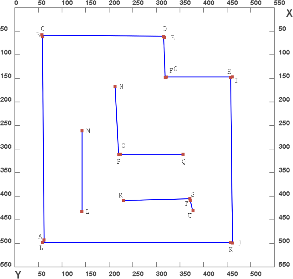
Test environment

Figure 9.

Noise point, border point and core point

Core point: These points form the interior of the density-based cluster. A point is a core point if the number of points within a given neighbourhood around the point as determined by the distance function and a user specified distance parameter, ε, exceeds a certain threshold, MinPts. In Figure 9, point A is a core point for the ε radius and MinPts ≤ 4.

Border point: A border point is not a core point but falls within the neighbourhood of a core point. In Figure 9, point B is a border point. A border point can fall within the neighbourhood of several core points.

Noise point: A noise point is any point that is neither a core point nor a border point and which does not satisfy the ε and MinPts criteria. In Figure 9, C is a noise point.

This section shows the results of applying DBSCAN clustering on LRF data to remove noise.

The values of ε and N_MinPts are set by training the robot and looking into the noise characteristics. The robot is trained in an actual environment based on user feedback. For a fixed value of N_MinPts, a maximum value is assigned to ε, i.e., ε=ε_max. The value of ε is consequently decreased - step by step - until a minimum ε_min is achieved, which gives an optimum noise reduction. Figure 8 shows the test environment where the robot was moved to collect the data points. Figure 7(a) shows the raw LRF data of the environment without removing noise. Figure 7(b) shows the result of DBSCAN applied on the raw data.

3.2.2 Noise removal using Mathematical Morphology

Morphology is a branch of mathematics which deals with a wide range of operators and which is particularly useful for the analysis of binary images. This section shows the applicability of these techniques on LRF data. The basic idea is to treat each point P_x,y obtained from the LRF as a pixel. Initially, the entire grid of size height × width of the setup environment is supposed to be null (i.e., zero). The points in the grid where the LRF data have a value greater than zero are treated as one. Next, we apply an erosion algorithm over the untreated scanned data. Details of the erosion technique can be found in various sources [26,11]. Erosion basically takes the logical AND operator of neighbouring data (which can be 0 or 1) to output the resultant data. In order to effectively apply an erosion technique over raw sensor data, this paper describes different kinds of kernels, which can be selected by the user according to the characteristics of noise. Each kernel is characterized by three parameters given by a logical vector:

V = {[\begin{matrix} \pm ψ_{H} & \pm ψ_{V} & \pm ψ_{C} \end{matrix}]}^{T}

(17)

Here, H, V and C represent the horizontal, vertical and crosswise (or diagonal) directions, respectively. Figure 10 shows the kernels DENSE × 3, PLUS × 4, PLUS × 8 and STAR × 8.

Figure 10.

Structuring element kernel type: (a) DENSE×3, (b) PLUS×4, (c) PLUS×8, (d) STAR×8. The central data point indicated in green is the point to be processed.

The raw LRF data (denoted by A) is viewed as a subset of the integer grid E = ℤ^dim where dim = 2. The raw data is probed with a predefined shape (structuring element, denoted by B) shown in Figure 10(b), which is a binary datum itself whose shape is defined by vector ψ_i where i ∈ H,V,C. For example, the structuring element B =PLUS × 8 (Figure 10(c)) is defined by:

ψ_{i} = \pm 2, i \in (H, V), ψ_{C} = 0

(18)

\begin{array}{l} E = Z^{2}; ​ B = {(- 2, 0), (- 1, 0), (0, 0), (1, 0), (2, 0), \\ (0, - 1), (0, - 2), (0, 1), (0, 2)} \end{array}

(19)

Erosion is defined by [38]:

A ⊖ B = {z \in E | B_{z} \subseteq A} ​ ​ o r ​ ​ A ⊖ B = \underset{b \in B}{\cap} A_{- b}

(20)

where B_z is the translation of vector B by vector z :

B_{z} = {b + z | b \in B}, \forall_{z} \in E

(21)

Erosion may also remove the actual data along with the noise. Although this may seem to be a drawback, in the case of LRF data it actually helps in data reduction for the faster computation of clustering described in Section 3.3. Some of the actual data lost by erosion can be obtained by performing a dilate operation, which is defined by:

A \oplus B = {z \in E | {(B^{S})}_{z} \cap A \neq Ø} ​ ​ o r ​ ​ A \oplus B = \underset{b \in B}{\cup} A_{b}

(22)

where B^S denotes the symmetric of B, i.e.:

B^{S} = {x \in E | - x \in B}

(23)

The kernels shown in Figure 10 are defined by the three parameters (ψ_H, ψ_V, ψ_C) summarized in Table 2. It is obvious that the kernel DENSE × 3 will remove more noise than the kernel PLUS × 4. Similarly, the kernel STAR × 8 will remove more noise than the kernel PLUS × 8. Since some actual LRF data also gets removed during the noise removal process, it is beneficial to actually try out and train the robot using different kernels in the actual environment. This can easily be done using the proposed framework, which is discussed in detail in Section 5. Figure 11(b) shows the results of noise reduction by Erosion using the PLUS × 4 kernel on noisy LRF data shown in Figure 11(a). Notice that some of the actual LRF data also gets removed, which can be recovered by applying dilation (the result of which is shown in Figure 11(c)).

Table 2.

Definition of various kernels with parameters

Fig.No.	Kernel Type	ψ_H	ψ_V	ψ_C
Fig. 10(a)	DENSE ×3	±1	±1	±1
Fig. 10(b)	PLUS ×4	±1	±1	0
Fig. 10(c)	PLUS ×8	±2	±2	0
Fig. 10(d)	STAR ×8	±2	±2	±2

Figure 11.

(a) Raw laser data of a wall with noise, (b) the erode operation, and (c) the dilate operation on (b)

Once the noise has been removed, clustering can then be applied in the spatial domain, which is discussed in the following section.

3.3 K-means and Fuzzy C-means Clustering

After removing the noise, clustering is applied on the noise-free LRF data. Clustering can be performed on real-time LRF data after each step in Online Mode or after a predefined N_{s_max} steps in Offline Mode. The choice of the mode of operation of the robot will also determine the number of clusters performed at each step. For Online Mode, the number of clusters (and hence the centroid) formed at each step is one, while for Offline Mode it can be greater than one (≤ 4 in our test environment). Either k-means or fuzzy c - means clustering is applied. A brief description of k-means and fuzzy c-means clustering is presented here.

k-means clustering [21,46,1] is a method of cluster analysis which aims to partition a set of data points into k clusters, such that each observation belongs to the cluster with the nearest mean. The k-means algorithm aims to minimize an objective function (a squared error function):

Q= \sum_{j = 1}^{k} \sum_{i = 1}^{n} {‖ p_{i}^{(j)} - c_{j} ‖}^{2}

(24)

Here, ${‖ p_{i}^{(j)} - c_{j} ‖}^{2}$ is a squared error distance measured between a data point p_i^(j) belonging to the j^th cluster and a cluster-centre c_j for n data points from their respective cluster centres.

The fuzzy c -means clustering [22, 1] (or ‘FCM’) is an extension of k-means clustering. FCM is similar to k-means clustering except that every data point in the data set is given membership by a weight ranging from 0 to 1, and each data point in the set belongs to every cluster with a weight (0 for does not belong at all, and 1 for absolutely belongs). The objective function that FCM optimizes is:

Q_{m} = \sum_{i = 1}^{N} \sum_{j = 1}^{C} u_{i j}^{m} {‖ p_{i} - c_{j} ‖}^{2} ​, ​ 1 \leq m \leq \infty

(25)

where m ∈ ℝ and m ≤ 1, u_ij denotes the degree of membership of p_i in the cluster j, p_i is the i^th r -dimensional measured data, c_j is the r -dimensional centre of the cluster, and ‖·‖ is the norm which expresses the similarity between any measured data and the centre.

The fuzzy partitioning of the data set is carried out by the iterative optimization of the objective function Q_m, with updated membership u_ij and cluster centres c_j by:

u_{i j} = \frac{1}{\sum_{k = 1}^{C} {(\frac{‖ p_{i} - c_{j} ‖}{‖ p_{i} - c_{k} ‖})}^{\frac{2}{m - 1}}} ​ ​, ​ ​ c_{j} = \frac{\sum_{i = 1}^{N} u_{i j}^{m} p_{i}}{\sum_{i = 1}^{N} u_{i j}^{m}}

(26)

the iteration stops when ${max}_{i j} {∣ u_{i j}^{k + 1} - u_{i j}^{k} ∣} < ν$ where ν is a termination criterion between 0 and 1, whereas k denotes the iteration steps. The process always converges to a local minimum or Q_m.

The implementation of the k-means and fuzzy c-means algorithms is straightforward using Equations (24), (25) and (26). Figure 12(a) and Figure 12(b) shows the result of applying k-means clustering and c-means clustering on noise-free TRF data with 52 clusters, respectively. The different colours applied to the TRF data clearly show the different clusters and have no other significance. The centroids obtained are also shown as circles in the case of k-means clustering and rectangles in the case of c-means clustering in Figure 12(a) and Figure 12(b), respectively. Later, these centroids are joined to form the map.

Figure 12.

(a) Results of clustering using k-means algorithm with 52 clusters, and (b) results of clustering using fuzzy c-means clustering algorithm with 52 clusters

3.4 Generating Straight-line Maps

If the centroids shown in Figure 12(a) and 12(b) are joined, exact straight-line maps may not be obtained as the centroids do not lie on the same slope. In some cases, it may be desirable to obtain straight-line maps. This can be solved by applying SVD to the centroids or by taking a Hough transform of the centroids. A brief description of both approaches is given in the following sections.

3.4.1 Applying SVD to the Centroids of the Clusters

A straight line can be obtained by applying SVD [30] on the matrix A which is composed of the centroids (c₁,c₂ … c_n) obtained after the clustering of the TRF data for a given θ :

A = [\begin{matrix} c_{1} \\ c_{1} \\ \cdot \\ c_{n} \end{matrix}]

(27)

The SVD of a matrix A is expressed as:

A = U S V^{T}

(28)

where U and V^T are orthonormal matrices consisting of the left and right singular vectors, and S is the diagonal matrix which is formed by the singular values arranged in decreasing order of the on-diagonal elements as follows:

U = [u_{1} \dots u_{n}]

(29)

S = [\begin{matrix} d i a g (σ_{1} σ_{2} \dots σ_{n}) \\ 0 \end{matrix}] (σ_{1} \geq σ_{2} \dots \geq σ_{n})

(30)

V = [υ_{1} \dots υ_{n}]

(31)

The matrices U and V satisfy U^TU = I and V^TV = I, where the matrix I represents the identity matrix.

The SVD calculations consist of evaluating eigenvalues and eigenvectors of AA^T and A^TA. The eigenvectors of A^TA make up the columns of V and the eigenvectors of AA^T make up the columns of U. Moreover, the singular values in S are square roots of the eigenvalues from AA^T or A^TA.

After computing the SVD of the centroids, the minimum (near-zero) singular values (σ) of the matrix S are ignored and set to zero. This is similar to the technique used in principal component analysis. The S_new with the smaller singular values ignored is then used to recalculate the matrix A_new consisting of points on the regression line as:

A_{n e w} = U S_{n e w} V^{T}

(32)

3.4.2 Applying a Hough Transform to the Centroids of the Clusters

A Hough transform is a technique for line extraction from binary images and its details are available in [12, 41]. The motivating idea behind the the Hough transform technique for line detection is that each input measurement (centroids in this case) indicates its contribution to a globally consistent solution. In the spatial domain, the straight line can be expressed as:

y = m x + c,

(33)

The equation of the line in the Hough space (ρ,θ) can be expressed as:

ρ = x \cos θ + y \sin θ .

(34)

The Hough transform algorithm is applied on the centroids obtained from k-means or fuzzy c-means clustering. After calculating the highest votes in the (ρ,θ) space, an inverse Hough transform is applied which gives the line passing through the maximum number of centroids. The Hough transform and inverse Hough Transform algorithm applied on the centroids is described in Algorithm 1.

Figure 13 shows the results of straight-line generation using SVD and the Hough transform on the centroids. The blue points represent the centroids of clusters obtained after the noise reduction and k-means clustering of a wide band of LRF data. The red line represents the line obtained after applying SVD. The green line represents the line obtained by using the Hough transform. It is clear from Figure 13 that SVD generates the regression line, whereas the Hough transform generates a line which passes through the maximum number of centroids. Since the number of clusters n_c is significantly less than the actual number of data points N (i.e., n_c << N), the Hough transform and the SVD are relatively inexpensive in terms of computation and memory in obtaining a straight line from the centroids.

Figure 13.

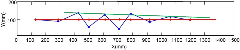
Straight-line generation from centroids using SVD and a Hough transform. The blue points represent the centroids, the red line represents the SVD line, while the green line represents the line obtained from the Hough transform.

Thus, the process of map generation in the spatial domain involves the following steps:

Gather LRF data in Online, Offline or Mixed Mode and segment data.

Remove noise by DBSCAN or mathematical morphological kernels.

Apply k-means or fuzzy c-means clustering.

Join centroids obtained after clustering.

Obtain straight-line maps by applying SVD or Hough transform to centroids.

The accuracy of the line maps obtained by joining the centroids around corners is affected by the number of clusters. One way to solve this problem is to increase the number of clusters. Furthermore, to overcome the extraction of the corners, other techniques like the split and merge [17, 48, 47] and IEPF [42] algorithms discussed earlier can be used.

4. Clustering in the Hough Domain (Accumulator Space)

The previous section discussed clustering in the spatial (i.e., xy) domain, in which clustering (k-means or fuzzy c - means) was directly applied to the LRF data after removing noise. It is necessary to first remove noise and then apply clustering because clustering is greatly affected by noise [35]. However, we can overcome this limitation by clustering in the Hough (ρ,θ) domain.

The Hough transform generates a straight line by looking into each LRF data point and, if there is enough evidence of an edge on that point, the Hough transform calculates the parameters for that line and increments the corresponding accumulator vote value [12, 41]. By finding the highest number of votes, or by looking for the local maxima in the accumulator space, the most-likely lines are extracted. However, with this method, votes which are even slightly lower than the threshold or the local maxima are ignored or else not taken into consideration while extracting the line. This is not good, especially when the data contains a lot of noise. Moreover, for long-range measurements, the noise increases for long-range sensors.

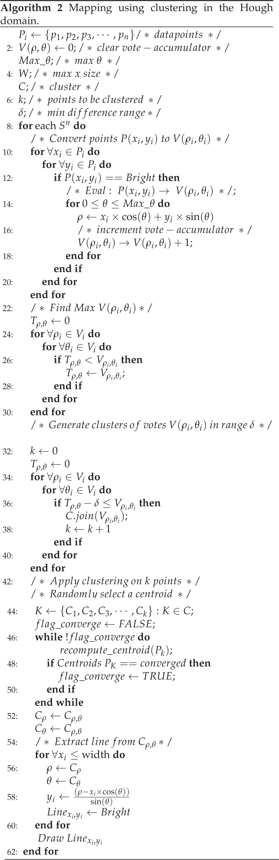
A Hough transform applied on a set of collinear points will converge at a single peak representing the highest number of votes in the accumulator space. Applying an inverse Hough transform on the peak point will generate a single straight line. However, in the real world, when the robot is moving, the LRF data is not collinear. An example of actual LRF data is shown in Figure 14(a). Applying a Hough transform on this LRF data will generate a Hough space, as shown in Figure 14(b), in which the (ρ,θ) curves do not intersect at a single point but rather at many intersecting points. Each intersecting point in the Hough space will correspond to a straight line which passes through one or more of the LRF data points. For the highest number of votes in the accumulator space, 13 green lines were produced, as shown in Figure 14(c).

Figure 14.

(a) Sample laser sensor scan data, (b) corresponding Hough space, and (c) single straight line (red) generated after clustering the Hough Space parameters. The red line is the optimum line obtained by clustering in the Hough domain.

Researchers have proposed many solutions [9, 44, 14, 23] for obtaining the most optimum parameter value by which a single straight line can be produced. Most of them are proposed for finding straight lines in real images for boundary or feature extraction. For the purpose of obtaining a single line for the LRF data, this paper proposes a new algorithm using the clustering of Hough space parameters.

To obtain a single straight line from the LRF data, we extend the voting procedure in the accumulator space to clustering. After getting the maximum vote value from the Hough space parameters (ρ,θ), clustering is applied to the accumulator votes which lie within a threshold in order to evaluate and compute a centroid. Generally, the highest vote value from the (ρ,θ) accumulator space is selected and a corresponding single line is obtained from that value. However, there are two problems with this approach. Firstly, there can be multiple points in the (ρ,θ) accumulator space with same highest-vote value. Each highest-vote value of (ρ,θ) will generate its own line, which will result in multiple line extractions. To get a single line for the purpose of building meaningful maps, the highest voted points are clustered and a centroid is obtained. The single line corresponding to the centroid point (ρ,θ) will receive contributions from all the highest voted points. Secondly, in a noise-free environment, the centroid of only the highest voted rho-theta (Vmax_rt) point can be calculated and a single line can be extracted to this point. However, for (ρ,θ) points whose vote value is slightly less than the highest vote (ex. Vmax_rt–1), these do not contribute to the final line and they are ignored when the environment is noisy. These slightly low voted points can also be taken into account while calculating the centroid, and the generated line will have contributions not only from the highest voted points but also from the slightly less voted points. This is shown in Figure 15. Figure 15(a) shows a sample lidar data scan with noise. Figure 15(b) shows the corresponding Hough voting space. The green line in Figure 15(a) is the line passing through the maximum number of points(corresponding to the highest vote value ‘6’, shown as a green dot in Figure 15(b)), and in a noise free environment this will be the desired line. The blue line is the line passing through slightly fewer points (corresponding to a vote value of ‘5’, shown as a blue dot in Figure 15(b)). In a noisy environment, this line should also contribute to the final result line. The red line represents the passing line corresponding to the centroid of the highest voted (ρ,θ) point with six votes and the slightly less voted point with five votes, shown as a red dot in Figure 15(b).

Figure 15.

Map generated using clustering in the spatial domain

Points with low votes generally correspond to noise and are not taken into account while clustering, and thus the effect of noise is greatly reduced particularly in the case of the LRF data. By taking the inverse Hough transform of the centroid, the most optimum line is obtained, which has contributions from the highest voted points. For the Hough space shown in Figure 14(b), the most optimum line obtained after the inverse Hough transform is shown in Figure 14(c) as a red line. Clustering can be done using k-means or fuzzy c-means clustering.

The algorithm is described in Algorithm 2. and explains the clustering of the Hough parameters using k-means clustering. For each segment of data Sⁿ obtained after applying segmentation described in Section 3.1, the algorithm begins by taking the Hough transform of the LRF data. Next, the highest vote value (denoted by T_ρ,θ) in the (ρ,θ) domain is found. In the next step, all the values of (ρ,θ) denoted by V_ρ,θ whose values are within the range δ (i.e., T_ρ,θ−δ ≤ V _ρ,θ) are extracted. Later, clustering is applied on the set of all such points and a centroid is obtained. Finally, the inverse Hough transform of the centroid point is taken to generate a line. The value of δ is generally set to ‘0’, ‘1’ or ‘2’. The higher values of δ will enable the clustering of (ρ,θ) points with lesser votes, which is not desirable. In the case of multiple lines, the LRF points corresponding to each line will be segmented into respective segments Sⁿ described in Section 3.1, where n is the number of lines. The Hough transform, clustering and inverse Hough transform are applied separately in each segment and lines are extracted. If P_iⁿ denotes the set of i vote points corresponding to the n^th segment S, then clustering is separately performed on the points in each segment, given by:

\begin{array}{l} p_{i}^{n} = {V_{ρ, θ}} (for each ​ ​ S^{n} separately), \\ \forall ρ, θ where T_{ρ, θ} - δ \leq V_{ρ, θ} \end{array}

(35)

For k-means clustering in the Hough domain, Equation (24) is used. In the case of Figure 15, Equation 35 represents two (ρ,θ) points with vote values of ‘6’ and ‘5’, shown as green and blue dots in Figure 15(b), respectively (δ = 1). Notice that the centroid obtained after clustering may or may not belong to the set of points denoted by Equation 35. For example, in the case of Figure 15, the centroid does not belong to the set of points given by Equation 35.

5. Framework

This section describes the framework for robot map building. The robot has a database, denoted by ‘Robot DB’ in Figure 16. This saves the kernels (Erode/Dilate, DBSCAN, k-means, fuzzy c-means, etc.). It also saves the temporary maps generated by the robot. The kernels can be updated by the server and the updated kernels are also saved in the database. The robot reads data from the LRF sensor which is then normalized. An appropriate kernel is selected from the database to remove noise. This can either be DBSCAN or Erode/Dilate or both, depending upon the instruction from the server. Before actually applying the kernel to the normalized data, a check is performed to see if the kernel is the most updated kernel. The necessary operation is performed (ex. Erosion and Dilation) and the resultant data is the input to the clustering algorithm, the Hough transform algorithm or other data-processing modules. The temporary map which is generated is saved in the robot database. The network module of the robot continuously polls to check if the temporary map has been updated and stored, and then transfers this map to the server for real-time display. This real-time display of the map at the server enables the tuning of the parameters of various kernels (e.g., select appropriate kernels or change the number of clusters). The server also has a database to store updated kernels.

Figure 16.

Framework for robot map building showing the robot side and the server side. The message is exchanged in xml format between robot and server.

The same network module is used to update the parameters or kernels of the robot which are stored in the robot's database. Since the robot continuously checks the database for updated parameters, they can be tuned from the server.

The message to update/tune the parameters kernel is carried out via an xml file which is parsed using an xml-parser by the robot to select an appropriate kernel and corresponding parameter values (ex. ε, minimum points in the case of DBSCAN, number of clusters). Listing 1 in the Appendix shows an example of such a message passed from the server to the robot. The xml message contains the instruction to select the DBSCAN noise removal kernel with 15 minimum points and an ε value of ‘5’. It also instructs the robot to remove noise using the PLUS × 4 kernel. The instructed mode is OnlineMode. The method of clustering is the k-means algorithm with two clusters. The straight line is to be generated by taking the Hough transform of the centroids.

6. Experimental Results

6.1 Test Environment

To test the accuracy and applicability of the proposed algorithms, experiments were performed in both an artificial test environment and a real cluttered environment. The artificial environment is shown in Figure 8. The artificial environment is made of straight polygonal walls. The robot was moved in a predefined path and laser data was collected. Random noise was added to test the algorithms. The real environment where the test was conducted consists of long straight corridors with narrow open spaces and cluttered with real objects. Figure 18 shows the panoramic view of the real environment. It is cluttered with objects with small narrow spaces for the robot to manoeuvre along. The experiments were performed on an Intel 1.8 GHz Core-i5 system with 4 GB RAM. The C++ language was used for framework implementation and the Java programming language was used for building the GUI.

Figure 17.

Map generated using clustering in the spatial domain

Figure 18.

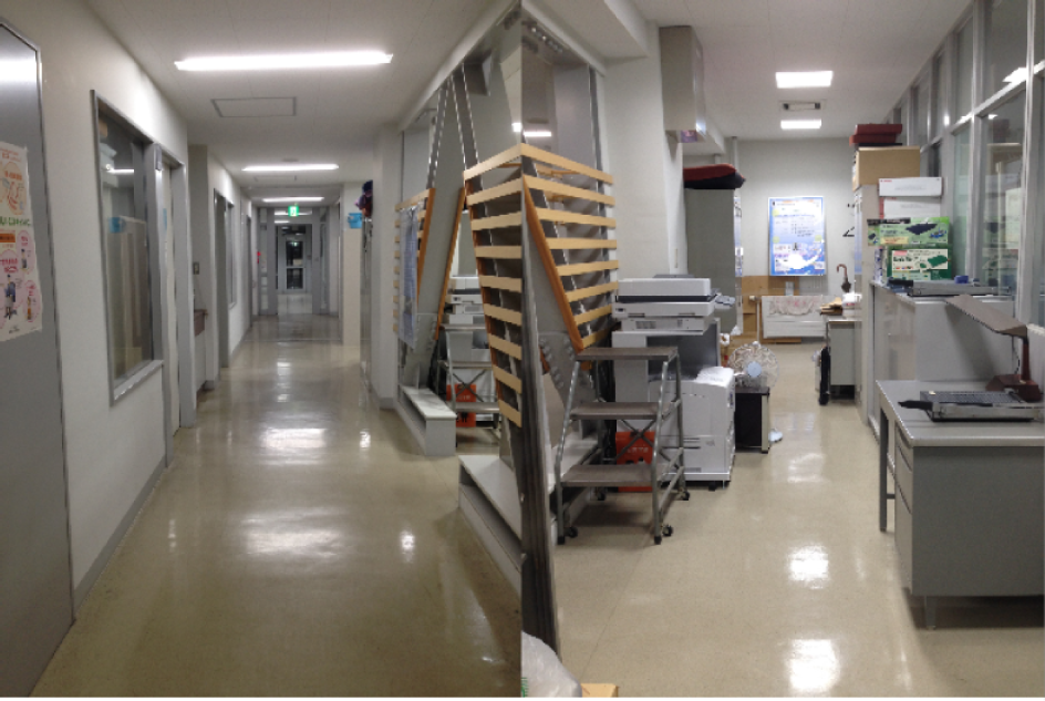
Panoramic view of a real test environment

6.2 Mapping Results

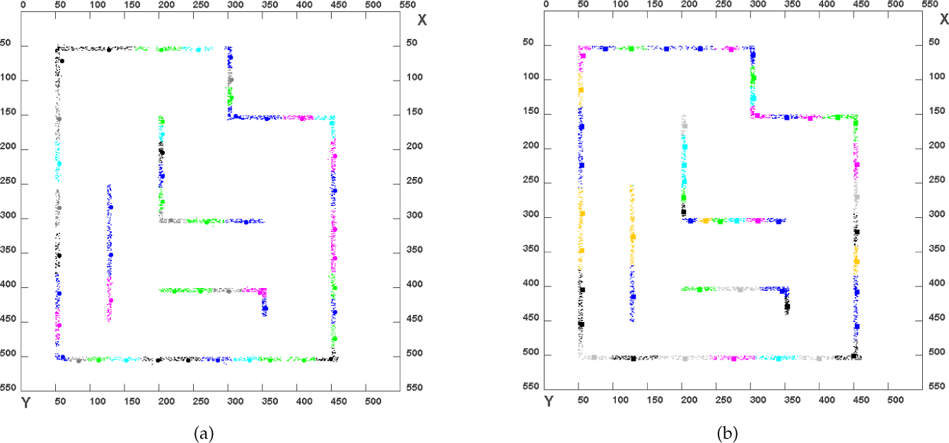
6.2.1 Artificial Test Environment

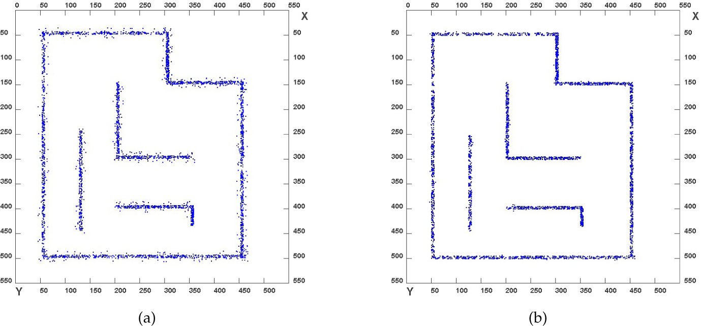
Figure 17 shows the final map generated after applying clustering (k-means and c-means) in the spatial domain on noise-free data as shown in Figure 7(b) with a varying number of clusters (30 to 70). Figure 19 shows the plot of the percentage error in an area of the map generated using k-means and c-means clustering with an increasing number of centroids. The percentage error is less than five percent with both types of clustering method. It can be seen that c-means clustering gives a slightly better performance compared to k-means clustering. However, the performance advantage diminishes as the number of clusters become larger. Figure 21 shows the final map generated from noisy LRF data as shown in Figure 7(a) using clustering in the Hough domain. We calculated the percentage error of the map area generated by clustering in the spatial domain by centroid joining, applying a Hough transform on centroids and by applying SVD on the centroids for 50, 60 and 70 clusters respectively. The results are summarized in Table 3. The fuzzy c-means clustering gives better results than the k-means clustering. Between the Hough transform and SVD on centroids, SVD gives slightly better performance. The plots of the scan position error and the odometry position error with respect to time are shown in Figure 20.

Table 3.

Percentage error of the map area for clustering in the spatial domain for an artificial environment as shown in Figure 8

No. of Cluster	50 clusters			60 clusters		70 clusters
Method	CJ	HT	SVD	CJ	HT	SVD	CJ	HT	SVD
k-means clustering	2.917	2.850	2.813	2.571	2.453	2.438	2.176	2.163	2.138
Fuzzy c-means clustering	2.621	2.510	2.450	2.240	2.215	2.188	2.002	2.343	2.05

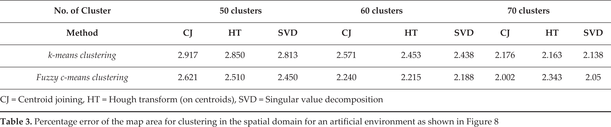
CJ = Centroid joining, HT = Hough transform (on centroids), SVD = Singular value decomposition

Figure 19.

Error plot showing the percentage in error with the number of clusters using k-means and fuzzy c-means clustering

Figure 20.

The plots of the scan position error and odometry position error with respect to time

Figure 21.

Map generated using clustering in the Hough domain

6.2.2 Real Environment

To test the robustness of our algorithms, experiments were performed in a real cluttered environment. The standard ICP technique [7] is utilized for fast scan-matching between consecutive scans obtained at different robot poses. In general, ICP is an iterative algorithm that iteratively finds the correspondence between two given scans and calculates a relative transformation that minimizes the distance between the corresponding points until the condition for termination is satisfied. A faster 2D version of the ICP method described in [24] is utilized in this study. For each iteration, it calculates the Euclidean squared distance between each and every possible combination of the registered points in two consecutive scans and finds the correspondence index based on the closest-point rule. The detected outliers are rejected as valid correspondences if their closest distance is above the given threshold. ICP-based localization was utilized in our experiments. The raw laser data for the environment is shown in Figure 22(a). The data has many outliers or noise. Figure 22(b) shows the result of applying DBSCAN on the ICP-corrected laser data. The noise from the raw data is removed after the applying DBSCAN. Figure 22(c) shows the result of applying k-means clustering. 160 clusters with their centroids are obtained. The clusters are shown in different colours. Figure 22(d) shows the simple polygon map which is obtained by joining the centroids from the k-means clustering. Figure 22(e) shows a line map generated by applying a Hough transform on the centroids obtained from the k-means clustering algorithm. The result shows straight line maps which are not affected by the cluttered environment. As the Hough transform is applied only on the centroid points, the process is relatively fast. Figure 22(f) gives the result after applying clustering in the Hough domain.

Figure 22.

Line maps obtained by the proposed algorithms

6.3 Comparison with Line Segment-based EKF-SLAM

The proposed algorithms are compared with standard line segment-based EKF-SLAM to check the applicability, improvements in processing time and accuracy of maps generated in an actual cluttered environment. Figure 23 shows the line map formed by EKF-SLAM. Due to the nature of the environment where the experiments are performed, noise present in the data affects the line extraction. It can be seen that multiple lines are generated due to poor feature association. Open areas are also not detected correctly and are wrongly associated with line features. EKF-SLAM generally suffers from poor data association because of an increase in uncertainty with increased numbers of features, especially in crowded and cluttered areas. In comparison, the proposed techniques are not affected by any of the above factors and they produce single lines and accurate maps as shown in Figure 22(d), Figure 22(e) and Figure 22(f), which represent the results of a map formed by joining the centroids, performing a Hough transform on centroids and clustering in the Hough domain, respectively.

Figure 23.

Map generated by line segment-based EKF-SLAM. The EKF robot trajectory is shown in green circles. The inset shows an enlarged part of the figure

6.3.1 Time Complexity

The time complexity of the proposed technique is compared with EKF-SLAM and the results are shown in Figure 24. EKF-SLAM is initially fast when the number of features is lower, but as the features increase, its complexity increases exponentially with time. This is expected as the feature number grows with time, and new features need to be associated by the EKF algorithm. For the complex environment, the uncertainty of the features also grows in the EKF algorithm. On the other hand, with the proposed technique, the map building process involves ICP matching, noise removal, clustering, line extraction and map correction. None of these steps requires complex feature association and, at each step, only the data that is available is processed. Compared to EKF, the proposed technique is slow, initially, but is more stable and in the long run as well as being more stable than the EKF. This makes the proposed method relatively stable for the entire 400 steps and it is much faster when compared to the EKF.

Figure 24.

Time cost between EKF-SLAM and the proposed technique

The time required by the robot to generate two clusters (in one step) for k-means & c-means were 26 ms and 38 ms, respectively. For noise removal, Erosion (15 ms) was faster than DBSCAN (28 ms), for one step of LRF data. ICP takes about (7 ms), as the robot does not make sudden rotations. Notice that the kernels employed for clustering and the mathematical morphological kernels were not optimized, and their implementation was straightforward. The framework was tested by changing the values of the number of clusters and the type of kernel. The robot stopped for approximately two to three seconds while the new parameters were being loaded.

7. Conclusion

This paper presented algorithms and a framework for generating maps in a noisy environment. The maps were generated using clustering techniques in the spatial and Hough domains. In the spatial domain, the algorithm first removes noise from the LRF data, for which we proposed to use density-based clustering and a mathematical morphological kernel of erosion. Afterwards, clustering was performed and the noise-free data and the centroids obtained were joined to form the map. The results show that straight-line maps with good accuracy can be generated by taking SVD or a Hough transform of the centroids. An algorithm for map building by clustering in the Hough domain was also proposed. Experimental results in both an artificial test environment and a real cluttered environment were performed and the results show that the proposed algorithms are very efficient for robot mapping in a noisy environment. We compared the results of the proposed technique with EKF-SLAM and showed that the proposed techniques can generate accurate single-line maps faster than EKF-SLAM for large datasets. Finally, we presented a framework to load the kernels or change the kernel parameters of the robot. The proposed framework makes it easy to change the kernels or fine-tune the parameters of the algorithms remotely based on live feedback.

Footnotes

8. Appendix

9. Acknowledgements

The present work is financially supported by MEXT (Ministry of Education, Culture, Sports, Science and Technology), Japan.

References

Jain

A.K

and Dubes

R.C.

Algorithms for clustering data. Prentice-Hall, Inc., Upper Saddle River, NJ, USA, 1988.

Ravankar

A. A.

Hoshino

Emaru

, and Kobayashi

Map building from laser range sensor information using mixed data clustering and singular value decomposition in noisy environment. In System Integration (SII), 2011 IEEE/SICE International Symposium on, pages 1232–1238, dec. 2011.

Ravankar

A. A.

Hoshino

Emaru

, and Kobayashi

Robot mapping using k-means clustering of laser range sensor data. Bulletin of Networking, Computing, Systems, and Software, 1, 2012.

Davison

A. J.

Reid

I. D.

Molton

N. D.

, and Monoslam

Stasse O.

: Real-time single camera slam. Pattern Analysis and Machine Intelligence, IEEE Transactions on, 29(6):1052–1067, June 2007.

Bandera

Perez-Lorenzo

J. M.

Bandera

J. P.

, and Sandoval

Mean shift based clustering of hough domain for fast line segment detection. Pattern Recognition Letters, 27(6):578–586, 2006.

Rao

Mullane

Wijesoma

W. S.

, and Patrikalakis

N. M.

Slam with adaptive noise tuning for the marine environment. In OCEANS, 2011 IEEE - Spain, pages 1–6, june 2011.

Segal

Haehnel

, and Thrun

Generalized-icp. In Proceedings of Robotics: Science and Systems, Seattle, USA, June 2009.

Fernandez

Moreno

Curto

, and Vicente

A. J.

Clustering and line detection in laser range measurements. Robot. Auton. Syst., 58:720–726, May 2010.

Fernandez

Moreno

Curto

, and Vicente

J. A.

Clustering and line detection in laser range measurements. Robotics and Autonomous Systems, 58(5):720–726, 2010.

10.

Premebida

and Nunes

Segmentation and geometric primitives extraction from 2d laser range data for mobile robot applications. Robotica, pages 17–25, 2005.

11.

Ronse

and Serra

Algebraic foundations of morphology. In Mathematical Morphology: From Theory to Applications, pages 35–80. ISTE / J. Wiley & Sons, 2010.

12.

Ballard

D. H.

Generalizing the Hough transform to detect arbitrary shapes. Pattern Recognition, 13(2): 111–122, January 1981.

13.

Sack

and Burgard

A comparison of methods for line extraction from range data. In In Proc. of the 5th IFAC Symposium on Intelligent Autonomous Vehicles (IAV, 2004.

14.

Walsh

and Raftery

A. E.

Accurate and efficient curve detection in images: The importance sampling hough transform. Pattern Recognition, 35(7):1421–1431, 2002.

15.

Davies

E. R.

Machine Vision: Theory, Algorithms, Practicalities. Morgan Kaufmann Publishers Inc., San Francisco, CA, USA, 2004.

16.

and Milios

Robot pose estimation in unknown environments by matching 2d range scans. Journal of Intelligent and Robotic Systems, 18(3): 249–275, 1997.

17.

Borges

G. A.

and Aldon

Line extraction in 2d range images for mobile robotics. J. Intell. Robotics Syst., 40:267–297, July 2004.

18.

Ahmad

and Namerikawa

Robot localization and mapping problem with unknown noise characteristics. In Control Applications (CCA), 2010 IEEE International Conference on, pages 1275–1280, sept. 2010.

19.

Durrant-Whyte

and Bailey

Simultaneous localization and mapping: Part i. Robotics Automation Magazine, IEEE, 13(2):99–110, June 2006.

20.

Cox

I. J.

Blanche-an experiment in guidance and navigation of an autonomous robot vehicle. Robotics and Automation, IEEE Transactions on, 7(2):193–204, Apr 1991.

21.

MacQueen

J. B.

Some methods for classification and analysis of multivariate observations. In Le Cam

L. M.

and Neyman

, editors, Proc. of the fifth Berkeley Symposium on Mathematical Statistics and Probability, volume 1, pages 281–297. University of California Press, 1967.

22.

Bezdek

J. C.

Ehrlich

, and Fcm

Full W.

: The fuzzy c-means clustering algorithm. Computers & Geosciences, 10(2):191–203, 1984.

23.

Jang

J. H.

and Hong

K. S.

Fast line segment grouping method for finding globally more favorable line segments. Pattern Recognition, 35(10):2235–2247, 2002.

24.

Martinez

J. L.

Gonzalez

Morales

Mandowand

, and Garcia-Cerezo

J. Mobile robot motion estimation by 2d scan matching with genetic and iterative closest point algorithms. Journal of Field Robotics, 23(1):21–34, 2006.

25.

Forsberg

Larsson

, and Wernersson

Mobile robot navigation using the range-weighted hough transform. Robotics Automation Magazine, IEEE, 2(1): 18–26, Mar 1995.

26.

Serra

Image Analysis and Mathematical Morphology. Academic Press, Inc., Orlando, FL, USA, 1983.

27.

Arras

K. O.

and Siegwart

R. Y.

Feature extraction and scene interpretation for map-based navigation and map building. In Proc. of SPIE, Mobile Robotics XII, pages 42–53, 1997.

28.

and Dellaert

Multi-level submap based slam using nested dissection. In Intelligent Robots and Systems (IROS), 2010 IEEE/RSJ International Conference on, pages 2558–2565, oct. 2010.

29.

Jixin

Kobayashi

Ravankar

A. A.

, and Emaru

Straight line segments extraction and ekf-slam in indoor environment. Journal of Automation and Control Engineering Vol, 2(3), 2014.

30.

Mathworks. Eigenvalues and singular values. http://www.mathworks.com/moler/eigs.pdf, Accessed: April 2014.

31.

Fischler

M. A.

and Bolles

R. C.

Random sample consensus: A paradigm for model fitting with applications to image analysis and automated cartography. Commun. ACM, 24(6):381–395, June 1981.

32.

Movafaghpour

M. A.

and Masehian

Poly line map extraction in sensor-based mobile robot navigation using a consecutive clustering algorithm. Robotics and Autonomous Systems, 60(8):1078–1092, 2012.

33.

Adams

M. D.

and Kerstens

Tracking naturally occurring indoor features in 2-d and 3-d with lidar range/ amplitude data. The International Journal of Robotics Research, 17(9):907–923, 1998.

34.

Ester

Kriegel

Jorg

, and Xu

A density-based algorithm for discovering clusters in large spatial databases with noise. In Proceedings of the Second International Conference on Knowledge Discovery and Data Mining (KDD-96), pages 226–231. AAAI Press, 1996.

35.

Laan

Pollard

, and Bryan

A new partitioning around medoids algorithms. Journal of Statistical Computation and Simulation, 73(8):575–584, 2003.

36.

Montemerlo

and Thrun

Simultaneous localization and mapping with unknown data association using fastslam. In ICRA, pages 1985–1991. IEEE, 2003.

37.

Engelhard

Endres

Hess

Sturm

, and Burgard

Real-time 3d visual slam with a handheld camera. In Proc. of the RGB-D Workshop on 3D Perception in Robotics at the European Robotics Forum, Vasteras, Sweden, April 2011.

38.

Soille

Morphological Image Analysis: Principles and Applications. Springer-Verlag New York, Inc., Secaucus, NJ, USA, 2 edition, 2003.

39.

Tan

Steinbach

, and Kumar

Introduction to Data Mining, (First Edition). Addison-Wesley Longman Publishing Co., Inc., Boston, MA, USA, 2005.

40.

Smith

R. C.

and Cheeseman

On the representation and estimation of spatial uncertainly. International Journal of Robotics Research, 5(4):56–68, December 1986.

41.

Duda

R. O.

and Hart

P. E.

Use of the hough transformation to detect lines and curves in pictures. Commun. ACM, 15(1):11–15, January 1972.

42.

Duda

R. O.

and Hart

P. E.

Pattern Classification and Scene Analysis. John Wiley & Sons Inc, 1 edition, 1973.

43.

Pfister

S. T.

Roumeliotis

S. I.

, and Burdick

J. W.

Weighted line fitting algorithms for mobile robot map building and efficient data representation. In In ICRA, pages 14–19, 2003.

44.

Guo

Pridmore

Kong

, and Zhang

An improved hough transform voting scheme utilizing surround suppression. Pattern Recogn. Lett., 30(13): 1241–1252, October 2009.

45.

Thrun

Burgard

, and Fox

Probabilistic Robotics (Intelligent Robotics and Autonomous Agents). The MIT Press, 2005.

46.

Kanungo

Mount

D. M.

Netanyahu

N. S.

Piatko

Silverman

, and Wu

A. Y.

An efficient k-means clustering algorithm: Analysis and implementation, 2000.

47.

Pavlidis

and Horowitz

S. L.

Segmentation of plane curves. IEEE Transactions on Computers, 23(8): 860–870, 1974.

48.

Nguyen

Gachter

Martinelli

Tomatis

, and Siegwart

A comparison of line extraction algorithms using 2d range data for indoor mobile robotics. Autonomous Robots, 23(2):97–111, 2007.

49.

Y. L.

Rad

A. B.

Chow

K. M.

, and Wong

Y. K.

Segment-based map building using enhanced adaptive fuzzy clustering algorithm for mobile robot applications. Journal of Intelligent and Robotic Systems, 35(3):221–245, 2002.

Algorithms and a Framework for Indoor Robot Mapping in a Noisy Environment Using Clustering in Spatial and Hough Domains

Abstract

Keywords

1. Introduction

2. Robot Odometry

3. Clustering in the Spatial Domain

3.1 LRF Data Segmentation

3.2 Noise Removal in the Spatial Domain

3.2.1 DBSCAN

3.2.2 Noise removal using Mathematical Morphology

3.3 K-means and Fuzzy C-means Clustering

3.4 Generating Straight-line Maps

3.4.1 Applying SVD to the Centroids of the Clusters

3.4.2 Applying a Hough Transform to the Centroids of the Clusters

4. Clustering in the Hough Domain (Accumulator Space)

5. Framework

6. Experimental Results

6.1 Test Environment

6.2 Mapping Results

6.2.1 Artificial Test Environment

6.2.2 Real Environment

6.3 Comparison with Line Segment-based EKF-SLAM

6.3.1 Time Complexity

7. Conclusion

Footnotes

8. Appendix

9. Acknowledgements

References