Sage Journals: Discover world-class research

Abstract

The existing skeleton extraction algorithms from a coarse and noisy model cannot achieve a satisfactory skeleton, let alone the joints' central position in a markerless motion capture system (e.g., a rigid skeleton). To solve this problem, we propose a rigid skeleton extraction algorithm from a noisy visual hull model with phantom volumes. Firstly, we reconstruct the subject visual hull and the corresponding volumetric model from a multiple-view synchronized video sequence. Secondly, the curve skeleton of the volume model is computed based on the theory of repulsive force fields. Thirdly, we propose a criterion for linking a curved skeleton to link the different skeleton limbs using a back-tracking method. At the same time, we obtain the distance and angle threshold values adaptively using a binary search algorithm. Finally, after achieving a smooth curve skeleton, we determine the joints' central positions in the skeleton using a priori information of the human body to form a rigid skeleton. Experimental results show that the proposed algorithm can obtain a desirable rigid skeleton with good robustness, less sensitivity to noise, and using an automatic procedure.

Keywords

Markerless Human Motion Capture Skeleton Extraction Rigid Skeleton Visual Hull

1. Introduction

Human motion capture is widely used in humanoid robot control [1], human-computer interaction [2], virtual reality [3], computer 3D animation production, video-based physical training, and gait analysis in medicine, etc. Consequently, 3D human motion capture based on a video sequence is one of the hottest research topics in computer vision and related applications. A traditional human motion capture system needs to place makers or sensors (such as LEDs, infrared sensors, magnetic sensors, rotation encoders or light-reflective markers) on the subject and transfer the position and motion trajectory of the markers to the computer. Next, the software analyses the data and produces the motion of the moving human body [3–5]. The traditional marker- or sensor-based system has some drawbacks: 1) the system is complicated, 2) it is hard to deal with the markers, 3) the markers will be occluded from view (which makes it hard to match the markers with the control points), and 4) it requires a lot of effort to post-process the motion data.

To overcome the above issues of the traditional motion capture system, an alternative approach would be a markerless human motion capture system using several synchronized cameras to capture the moving subject in the scene, reconstructing the 3D model of the human from the video sequence, and then recovering the human motion, including the positions of the joints and the angles of rotation of the body [6, 7]. In the multi-view scenario,

according to how the human models being used, markerless human motion capture methods (also called ‘pose estimation algorithms’) can be divided into three categories: 1) model-free methods, which do not employ an a priori model [8, 15], 2) reference model-based methods, which use a reference to constrain and guide the interpretation of the measured data [9, 10], and 3) a model which is a representation of the observed subject, maintained and updated over time and which can provide any desired information regarding pose and location [11, 12]. Among these methods, one of the most important 3D representations is the 3D human skeleton, especially a rigid skeleton with information about the joins' central positions, representing the human motion status at a given moment. Generally, the visual hull model (an outer approximation of the subject from a silhouette image sequence) is an initial estimation of a moving subject. However, one of the main problems from which the visual hull model suffers is the presence of phantom volumes due to view occlusion of the cameras (see the two examples in Fig.1 [1, 21). As such, it is not a trivial matter to extract the skeleton from these noisy artefact visual hull, which are created by the traditioni. mesh-based method.

Figure 1.

Visual hull models with phantom volumes

In this paper, we focus on the study of 3D rigid skeleton extraction from a visual hull model with noise and a phantom volume for a markerless human motion capture system.

2. Related Work

The skeleton extraction algorithm is a well-studied topic in computer graphics. Voronoi graph-based methods are commonly used [13, 14]. C. Menier [19] et al. determine the noisy medial-axis of a human model using an algorithm based on Voronoi graphs. Next, in order to obtain the kinematics skeleton, they match the noisy medial-axis with i the pose space using maximum likelihood and EM optimization approaches. In addition, many researchers use a skeleton extraction algorithm based on topology thinning [20, 21]and Reeb graphs[22–25].

Zhuang et al. [26] propose a method to capture motion from video using feature tracking and skeleton reconstruction. Based on a Kalman filter and a morph-block similarity algorithm, every part of the human body from top to bottom is tracked. Using the camera calibration parameters and the prior model, the 3D motion skeleton is established. Chu [15] et al. transform the human volume in a Euler space into a pose-invariant intrinsic space using Isomap. In this intrinsic space, the non-linearity caused by the rotation of a human joint can be reduced and the skeleton extraction can be simplified. After the principle curves have been determined, it is recovered as the skeleton in the Euler space through the use of interpolation. Yu et al. [27] extract the 3D human skeleton according to Mores' geodesic distance theory. This algorithm could achieve good results, and it can extract the skeleton of the 3D human model in various poses created by the scanner. However, it is highly sensitive to the noise of the model boundary; hence, it shall not be used to extract skeleton from the visual hull with a low accuracy. O.K.C. Au [28] et al. extract the skeleton using the mesh contract algorithm, which is very fast. However, it is highly sensitive to the noise of the model boundary.

Takahashi et al. [17] propose a markerless human motion capture system from volumetric data with a simple human model. In this method, an articulated cylindrical human model is introduced into the human body posture estimation system in order to obtain 3D skeleton information about a human body. Firstly, the volumetric model is created through the commonly used back projection method. By fitting the cylindrical model to the reconstructed human body in a 3D volume as a set of voxels, the skeleton can be obtained as a set of cylinder axes. As the cylindrical model is used to fit the volumetric data, this approach is not accurate enough to represent the skeleton.

Oda et al. [29] extract the skeleton from a 3D model by using geodesic distance theory. This kind of algorithm adds more or less manual operations and simplifies the model, reducing the total computation time. C. Theobalt [16] et al. fit the volume model with various hyper-polyhedrons and then determine the hyper-polyhedrons' centre positions as the skeleton joint following splitting and merging operations. The merit of this algorithm is that an a priori skeleton model is not necessary, although the drawback is that splitting and merging process takes too much time, in addition to the fact that it is hard to find a suitable error criterion. In [30], they present a volumetric data-based human skeleton extraction approach based on a skeletal graph. The differences between this method and ours are that: 1) the subject is assumed to be standing upright, and 2) it uses 10 cameras (which is more than our system). That means that the visual hull model is much cleaner than that used by our method. [32] and [33] also belong to the category of volumetric model-based methods. These two kinds of algorithms are similar, and can give good performance for the models with a high degree of accuracy and less noise. The normalized gradient vector flow-based algorithm [33] can only produce a discrete voxel skeleton instead of a curve skeleton. On the contrary, the repulsive force-based approach can provide a good curve skeleton from volumetric data, which can be used to further extract the rigid skeleton.

To summarize, the drawbacks of a rigid skeleton extraction algorithm from a 3D human visual hull model include: 1) they require too much manual intervention, 2) they are sensitive to the noise of the model, 3) they cannot determine the joints' centre positions accurately. To settle the above problems, we propose a 3D model rigid skeleton extraction algorithm which needs no manual intervention and which is not sensitive to the model noise or phantom volumes. Firstly, we compute the repulsive force vector field of a 3D human volumetric dataset, determining the curve skeleton. Secondly, we analyse the positions and slopes of the skeleton curve, linking the disorder skeleton point into smooth curves using the back tracking and binary search methods. This skeleton extraction algorithm reduces the sensitivity to noise, using anthropological knowledge to determine the joints' position in the human model. Experiments show that this algorithm exhibits good effectiveness and robustness.

3. Algorithm Overview

The whole process of this skeleton extraction algorithm comprises three parts: 1) curve skeleton extraction, 2) skeleton linking, and 3) localization of the joints' centre positions. Firstly, we reconstruct the volumetric data of the human from multiple-view synchronized videos. Secondly, we calculate the curve skeleton based on repulsive forces from a volumetric dataset. Next, we propose a linking criterion to link and smooth each skeleton limb using a back tracking strategy and find the adaptive angle and distance threshold values using a binary search algorithm when we link the skeleton. After obtaining the smoothed skeleton, we ensure that the limbs of the skeleton are self-correcting so that they fit the volume modal well. Finally, we calculate the joints' centre positions according to the length and proparty relations of the given observation model. Figure 2 shows the entire pipeline of processing one subject to generate a rigid skeleton.

Figure 2.

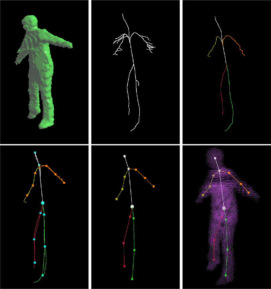
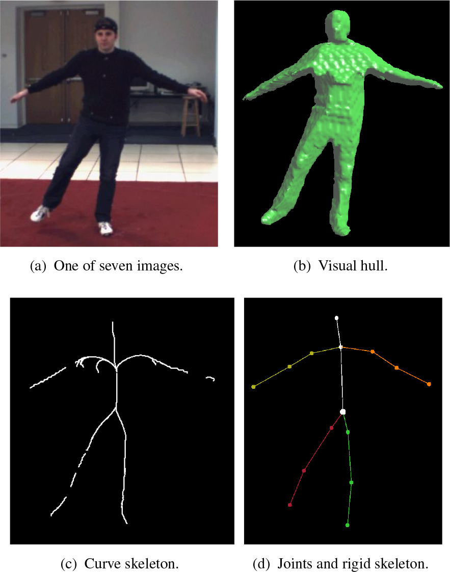
Work flow of our rigid skeleton extraction algorithm from a noisy visual hull: (a) one of the frames from the multi-view videos, (b) a silhouette extracted from the image, (c) the visual hull model, (d) the volume model, (e) the estimated curve skeleton from (d), (f) the smoothed curve skeleton, and(g) the rigid skeleton with the joints' positions

4. Curve Skeleton Extraction

4.1 Computation of the Volume Model

In this section, we describe the volume data reconstruction algorithm based on multiple calibrated cameras. The multiple-view video sequence database we use is HumanEve [18], which is from the computer college lab of Brown University. This database is specialized for the testing of motion capture systems. HumanEve supplies seven views of synchronized video as well as calibration parameters, including intrinsic parameters and external parameters for each camera. With these calibration parameters, we can build an initial 3D bounding box of the human body. We calculate the bounding box from a set of silhouettes and the projection matrices. Firstly, the 2D bounding boxes for each silhouette are computed and then back-projected. The bounding box of the subject can be obtained by an optimization method for each of the six variables (x_min,y_min,/z_minandx_max,y_max,z_max,) defining the bounding box [31].

After acquiring the 3D bounding box, we divide the space into N x N x N voxels within the volume and project each voxel onto each image. If one point falls within the entire image foreground, it is marked as a voxel of a human model. Otherwise, if one point falls outside of at least one image foreground, it is not marked as a voxel. After the projection test, we are able to obtain a volume model of the subject. Song et al. [31] also use an octree structure to store the volume data. Since this part of job is not the focus of this paper, we will not provide a detailed introduction, and readers mayreferto[31].

4.2 3D Curve Skeleton Extraction

We describe the boundary voxels on a human model as each unit point charge. Next, we calculate the repulsive force of each point inside the model by charging the object's boundary to generate a repulsive force field. Next, the topology characteristic of a repulsive force vector field, such as the convergence point or the saddle point [32], is analysed. Finally, a hierarchical curve skeleton is extracted according to these topology characteristics.

4.2.1 Core Skeleton

We give, here, a definition of repulsive force. Let C be a unit point charge from which the repulsive force F_pc of any point P in a volume model is inversely proportional to the n th power of the distance R. The direction of the repulsive force is from C to P:

F_{p c} = \frac{C P}{R^{n}}

(1)

where CP is the normalized vector from C to P, n = 1,2,…, called the ‘order of repulsive force’ function. The composition of repulsive forces from each point on the model boundary to the unit point charge P is:

F_{p} = \sum_{i} F_{p c_{i}}

(2)

where F_pci is the repulsive force on point P which is from the unit point charge C_i. F_p is the composition of the repulsive forces from each boundary unit point charge C_i.

For each point in the volume model, the composition of its repulsive forces from the boundary points is calculated and a 3D repulsive force vector file is formed. Next, we extract the curve skeleton of the model according to the topology characteristics of the repulsive force field. In this repulsive force field, the critical points are very important for curve skeleton extraction. The critical points are those points where the repulsive force vanishes. There are three types of critical points: 1) a convergence point, where all the force vectors in its neighbourhood are directed to it, 2) a repulsive point, where all the force vectors in its neighbourhood deviate from it, and 3) a saddle point, whereby some of the force vectors are directed to it and others depart from it. Since the saddle points exist between the convergence points and the repulsive points, we can thus use saddle points to link the convergence points with the repulsive points.

From each saddle point, we can link the points following the directions of the eigenvectors of the Jacobian matrix of the vector file at the critical point in the two opposite directions until meeting the convergence point and the repulsive point [32]. The curve formed by these critical points is called a ‘critical skeleton’. The curve forms the core skeleton of the 3D volume model.

4.2.2 Low Divergence Point and Level 2 Skeleton

The divergence of the vector flow is defined as:

d i v F = \nabla \cdot F = \frac{\partial F_{x}}{\partial x} + \frac{\partial F_{y}}{\partial y} + \frac{\partial F_{z}}{\partial z}

(3)

where F_x, F_y and F_z express three components in a three-axis orientation of the repulsive force, respectively. When the value of divF is relatively small, its topology characteristic represents a “sink” [32]. Those points for which the divergence is below a given threshold can be marked as the new seed points for forming the skeleton. These seed points should be linked with the core skeleton and they form a new skeleton. With the various threshold values, different numbers of seed points will be calculated and skeletons of different densities will be formed. The larger the threshold is, the greater the number of seed points that will be obtained and the greater the number of skeleton points that will be created. Experiments show that the best resultis achieved when n=3.

4.3 Algorithm Pipeline

The algorithm presented above can be summarized as:

Calculate the boundary points of the model.

For each point in the model, calculate its composition repulsive force from the boundary points and form a repulsive force vector field.

Calculate the critical points, determine the critical curve and form the core skeleton.

Calculate the divergence of the force field and choose the points with low divergence as new seed points to form a new skeleton.

Figure 3 reveals a comparison of the extracted skeleton using the repulsive force-based method and mesh contraction [28]. From these two figures, we can see that the force repulsion-based method can maintain the topology structure and that it has fewer noise bifurcations due to the non-sensitivity characteristic of the boundary noise of the mesh model.

Figure 3.

Curve skeleton from the repulsion force method and the mesh contraction-based method

5. Rigid Skeleton Creation

5.1 Determine the Torso

We first calculate the centre of gravity of the whole volume model and then determine the closest approach point from the gravity centre, in the curve skeleton. The closet approach point is the torso of the volume model. In practice, the position of the torso centre closes to the belly button, demonstrated in Figure 4 (the black point). The centre of gravity is computed by $P_{c g} = (x_{c g} = \frac{\sum_{i = 1}^{N} x_{i}}{N}, y_{c g} = \frac{\sum_{i = 1}^{N} y_{i}}{N}, z_{c g} = \frac{\sum_{i = 1}^{N} z_{i}}{N})$ , where (x_i, y_i,z_i) is the ith voxel and N is the total number of non-empty voxels. If the subject stands upright,

Figure 4.

Torso position approximation via the centre of gravity. The right-hand figure is a zoomed portion of the torso position.

we can consider that the point (x_cg,y_cg,z_cg) is the torso point.

However, when the pose of the human body is arbitrary (such as when stooping, kicking, etc.), the centre of gravity will deviate away from the real torso position. In order to get an accurate torso location, we use the following strategy to locate a more stable and accurate torso point.

Compute the curve skeleton points in a neighbourhood of P_cg, denoted as P_nbh, e.g., S_nbh = {P|P ∈ S, dP,P_cg)<ε}, where e is the radius of the neighbour, S is the curve skeleton set, and d(·, ·) is the distance between P and P_cg.

Calculate the distance in set S_nbh and eliminate the points with the greatest distance.

Recompute the centre of gravity in the rest points in set S_nbh (this centre of gravity looks like the torso position - see the zoomed portion in Figure 4).

5.2 Linking the Skeleton

Since the curve skeleton consists of various skeleton segments, it is highly disordered, as shown in Figure 5. Hence, the lower limbs and the backbone, will be linked separately in order to get smooth skeleton segments. Thus, a linking criterion should be defined. That is, given a point as a start point, how do we find a path whereby all the points in the path form a smooth skeleton?

Figure 5.

Skeleton combo of frame 1, 500 of the S3 model in the HumanEve database

5.2.1 Skeleton Linking Criterion

The intersection angle of the skeleton section line is the intersection angle of two distinct lines formed by any two distinct points on the skeleton. For example, the intersection angle between line AB and line BC is shown by eq. (4):

\begin{array}{c} 〈 \vec{A B}, \vec{B C} 〉 = \arccos \frac{\vec{A B} \cdot \vec{B C}}{∥ \vec{A B} ∥ ∥ \vec{B} C ∥} \\ = \arccos \frac{x_{a b} \cdot x_{b c} + y_{a b} \cdot y_{b c} + z_{a b} \cdot z_{b c}}{\sqrt{x_{a b}^{2} + y_{a b}^{2} + z_{a b}^{2}} \cdot \sqrt{x_{b c}^{2} + y_{b c}^{2} + z_{b c}^{2}}} \end{array}

(4)

where || · || represents the norm of the vector.

Suppose we start from p oint A. If the next point of A is its closest point B, then the next point of B - if it exits, and supposing that it is point C - must satisfy the conditions below:

C ∈ N_r(v)={P|P∈S, P≠B, d (P, B)<r}, where S is the set of skeleton points d(P₁,P₂) represents the Euclidean distance between P₁ and P₁ and P₂ represents the radii of the neighbourhood of B.

Angle $〈 \vec{A B}, \vec{B C} 〉 < a n g T h r$ , where angThr, is the threshold of the angle.

In the neighbourhood of B, if there is more than one point, the closet point from B is set to be the next point of B, marked as C. Next, start from point C in order to find its next point using the same procedure until there is no point satisfying the conditions or else meeting the given ending point. Suppose that the next point of the skeleton point A is B, as shown in Figure 6, and that C and D lie within the neighbourhood of B. d(B, D)<d(B, C), but $〈 \vec{A B}, \vec{B C} 〉 < 〈 \vec{A B}, \vec{B D} 〉$ , which shows that point C is more reasonable than point D tobe the next point of B. In fact, given a different combination of distance thresholds and angle thresholds, the noise annoyance level will be different and the path will also be different.

Figure 6.

A sketch map of a linking criterion

5.2.2 Steps of the Algorithm

We use the back-tracking algorithm to link each skeleton segment. Given an initial combination of distThr and angThr, let the start point startPt be the current point, calculate its closet point set by using the Kd-trees algorithm [34], and determine its next point according to the linking criterion described in Section 5.2.1. If a further point is obtained, push the current point into a stack and let this further point be the current point, and then repeat the same steps. If the given ending point is successfully found, the linking is successful - reduce the distance threshold and angle threshold. Otherwise, popping the current point from the stack and continue linking. If the given ending point cannot be reached in all cases, the linking fails - enlarge the distance threshold and angle threshold, and repeat linking. We use a strategy similar to a binary search to find a proper combination of the distance threshold and the angle threshold. For each combination, we test the linking result continuously, narrowing the search range continuously to avoid the traversal of the whole search space, thereby reducing the calculation time.

To take the linking of the lower limbs, for instance, the procedure of the algorithm is described as below:

Step 1: Select an initial combination of the distance threshold distThr and the angle threshold angThr.

Step 2: Select a start point (when linking the lower limbs, set as lowest point) as the start point startPt, and let the torso be the ending point endPt.

Step 3: Let starPt be the current point curPt, and calculate its neighbourhood with a radii of distThr.

Step 4: If there is no point in the neighbourhood meeting the constraint condition of the distance and the angle, turn to Step 5; otherwise, turn to Step 6.

Step 5: If the stack path is empty, let flag isSuccess = false, and turn to Step 8; otherwise, pop the curPt from the stack path and turn to Step 3.

Step 6: Push curPt into the stack path, remove curPt from the skeleton point set, mark the next point as the current point and turn to Step 3.

Step 7: If the given ending point is reached, let flag i sSuccess = true and turn to Step 9.

Step 8: Adjust the distance threshold distThr and the angle threshold angThr, and turn to Step 1.

Step 9: End.

5.2.3 Segment Curve Skeleton

In order to obtain the accurate centre positions of the joints, we should segment the curve skeleton as the backbone, the two upper limbs and the two lower limbs. First, we calculate the lowest point as the start point and let the torso be the ending point, and link the skeleton according to the linking criterion described by Section 5.1, forming one leg. We can also link the other leg with the same steps. Second, we calculate the highest point as the start point and let the torso be the ending point, such that we can link the backbone. Next, we prune the backbone and the two lower limbs. In this new set of left-skeleton points, we calculate the farthest point from the backbone as the candidate of one wrist. For the whole curve skeleton, we mark these candidate points as start points and the torso as the ending point, linking the skeleton. The longest two paths are the upper limbs. The linking order is as follows:

Spine: Torso → Neck → Head.

Lower limbs: Torso → Left/right ankle → Left/right knee → Left/right hip.

Upper limbs: Lrft/right shoulder → Left/right elbow → Left/righg wrist.

Figure 7 is an example of curve skeleton segmentation for the firth frame of the S2 model in the HumgnEva dataset.

Figure 7.

An example of curve skeleton segmentation: frame two of the S2 model in the HumanEve database

5.3 Determine the Joints Positions

We obtained the smoothed and segmented curve skeleton of the limbs - shown in Figure 7 - according to the last section. Next, we must determine the joints' centres. For a given human model, the lengths of each limbs are known [18] and so we can determine the joints' positions in the curve skeleton by the length of each limb.

From the torso centre, calculating the distance between this point and other points in the backbone, until the distance equals the prior length, the neck position is determined. However, in most cases, the joint does not lie on the curve skeleton but rather in the interval of the tow points. Next, the accurate position of joint should be calculated by linear interpolation. Using the same method, the positions of the head, the hips, knees and shoulders are determined.

In the curve skeleton obtained by the repulsion force field theory, the shoulders do not fit the real human body well, and so they need adjustment. First, the vector JN from the joints of the backbone and the upper limbs to the neck is calculated; next all the points Pn,i(xn,i yn,i,zn,i) ∈ Sn, upLimb i = 0,1,2,…, (size(Sn,upLimb)- 1,n ={1,2} representing the two upper limbs) of the two upper limbs in the curve skeleton are moved to new positions according to eq. (5):

{\begin{array}{l} {x^{'}}_{n, i} = x_{n, i} + X_{J N} \cdot {(\frac{L_{n} - l_{n, i}}{L_{n}})}^{m} \\ {y^{'}}_{n, i} = y_{n, i} + Y_{J N} \cdot {(\frac{L_{n} - l_{n, i}}{L_{n}})}^{m} \\ {z^{'}}_{n, i} = z_{n, i} + Z_{J N} \cdot {(\frac{L_{n} - l_{n, i}}{L_{n}})}^{m} \end{array}

(5)

where P'n,i(x'n,i,y'n,i z′n,i) represents the new positions, L n(n = 1,2) represents the total length (i.e., the geodesic distance) of the upper limbs, and ln,i represents the geodesic distance between the i th points in the n th upper limb to the joints of the backbone and the upper limb:

l_{n, i} = d (J o i n t, P_{0}) + d (P_{0}, P_{1}) + \dots + d (P_{i - 1}, P_{i})

(6)

where $i = 1,2, \dots, s i z e (S_{n, u p L i m b}) - 1, X_{J N}, Y_{J N}$ and ZjN represent each component of the vector $\vec{J N}$ , m represents the order of the mathematical equation. Eq. (6) causes a translation of the upper limbs along with the vector $\vec{J N}$ , with a translation range of $(0, ‖ \vec{J N} ‖]$ . The closer it is to the backbone, the further it moves. The experiments show that, when m =3, it gives a satisfactory performance, as shown in Figure 8.

Figure 8.

The processes of adjusting the upper limbs of frame five of an S2 gesture: (a) curve skeleton segmented, (b) curve skeleton and volume model, (c) curve skeleton after adjusting the upper limbs, (d) curve skeleton and volume model

6. Experimental Results

The implementation of the algorithm is made on a PC platform comprising a Pentium IV 3.0 GHz with 1.25 G memory, Windows XP OS, the OpenGL graphics library and the Visual C++ programming environment. The sets of human models in the HumanEva database are chosen.

In Figure 9, the visual hull (a) is constructed from seven images of S2 gesture data, and then the raw curve skeleton (b) is determined by the theory of repulsive force fields. Afterwards, it is linked and segmented, the smooth curve skeleton (c) is obtained, the joints are determined and the upper limbs are adjusted(d). Finally, the rigid skeleton (e) with the joints' centre positions fitting the volume model (7) is calculated. Correspondingly, Figure 11 gives the results of frame 1, 500 of the S3 combo data. The resolution of the volume observation model is 128times128times128. The observation model is not as smooth or as precise as the 3D scanning model, since the volume and the mesh model are constructed from seven synchronization video sequences with inadequate information, and the 3D reconstruction algorithm itself has some shortcomings. Consequently, there is some noise in the curve skeleton as calculated by the repulsive force field theory, such as for the lower limbs and the abdomen as shown in Figure 9. Figure 10 and Figure 12 are the side view of the visual hull, the curve skeleton and the final rigid skeleton.

Figure 9.

Rigid skeleton extraction from a noisy visual model, taking frame two of the S2 model in the HumanEve database as an example (front view)

Figure 10.

Rigid skeleton extraction from a noisy visual model, taking frame two of the S2modelintheHumanEve database as an example (side view)

Figure 11.

Rigid skeleton extraction experiment from frame 1, 500 of the S3 model in the HumanEva dataset (front view)

Figure 12.

Rigid skeleton extraction experiment from frame 1, 500 of the S3 model in the HumanEva dataset (side view)

The linking algorithm that we propose can link the skeleton segments with good performance and smooth the curve skeleton. The curve skeleton can be adjusted automatically to fit the real human skeleton well by using eq. (6) (Figure 9(d)). The experiments with the S3 combo data (Figure 11) also show that the skeleton extraction algorithm proposed in this paper can extract the skeleton of the observation models reconstructed from multiple-view synchronization video sequences with satisfying results. To verify the robustness of this algorithm, we conduct an experiment of successive frames of the S3 combo video. For ease of presentation, we test every 80 frames of the video sequence. The results are shown in Figure 13, Figure 14 and Figure 15, from which we demonstrate the robustness of our algorithm.

Figure 13.

Rigid skeleton extraction experiment from frame 1, 520 of the S3 model in the HumanEva dataset

Figure 14.

Rigidskeleton extraction experiment from frame 1, 600 of the S3 model in the HumanEva dataset

Figure 15.

Rigid skeleton extraction experiment from the frame 1500 of S3 model in HumanEva dataset

7. Conclusion

Many skeleton extraction algorithms derived from a coarse or a noise model could not achieve a satisfactory skeleton. The main contribution of our paper is that a new method is presented to extract the rigid skeleton from a noisy visual hull model. Firstly, we propose a criterion for linking the curve skeleton with different skeleton limbs using a backtracking method. At the same time, the distance and the angle threshold values can be adjusted automatically to form a smooth curve skeleton. Hence, the 3D skeleton extraction algorithm's sensitivity to the noise of the model boundary is reduced and its robustness is good. We test successive frames of the video sequence and achieve a satisfactory curve skeleton and a rigid skeleton from the volume model. Secondly, we propose a method for calculating the joint positions automatically. This algorithm can determine the joint positions without any manual marking. It can be used in the initial pose estimation of a markerless human motion capture system and for self-recovery when tracking fails. The results show that our algorithm can obtain a desirable result as well as good robustness, and also that it can reduce the 3D skeleton extraction algorithm's sensitivity to the noise of the model.

However, at present, one of the limitations of our proposed method is that its computational efficiency cannot meet the requirements of real-time applications, since the computational complexity of the algorithm is O(N³), where N is the number of object voxels - more than one second is used to process one frame. Our future work will be to accelerate the algorithm with a parallel computation technique as this algorithm is intrinsically suitable to be processed in parallel.

Footnotes

8. Acknowledgements

This project is partially supported by the Science & Technology asic Research Projects of Shenzhen (No. JC201104210015A, JCYJ20140417172417166, CYZZ20140829101945536).

References

Theobalt

Magnor

Schueler

Seidel

H.P.

. (2002) Combining 2D feature tracking and volume reconstruction for online video-based human motion capture (PDF). In: Proceedings of Pacific Graphics, Beijing, China. 96–103.

Kilner

Starck

Guillemaut

J.Y.

Hilton

. (2009) Objective quality assessment in free-viewpoint video production, Journal of Image Communication, 24(1-2): 3–16.

Moeslund

T.B.

Granum

. (2001) A survey of computer vision-based human motion capture, Computer Vision and Image Understanding, 81: 231–268.

Picerno

Cereatti

Cappozzo

. (2008) Joint kinematics estimate using wearable inertial and magnetic sensing modules, Gait & Posture, 28: 588–95.

Collins

T.D.

Ghoussayni

S.N.

Ewins

D.J.

(2009) A six degrees-of-freedom marker set for gait analysis: Repeatability and comparison with a modified Helen Hayes set, Gait & Posture, 30: 173–180.

Pansiot

. (2009) Markerless visual tracking and motion analysis for sports monitoring, PhD Thesis.

Rosenhahn

Schmaltz

Brox

(2008) Markerless motion capture of man-machine interaction, IEEE Conference on Computer Vision and Pattern Recognition, 2008, Jun. 23-28, Anchorage, Alaska, USA, 1–8.

Agarwal

Triggs

. (2004) 3D human pose from silhouettes by relevance vector regression, Proceedings of the IEEE Conference on Computer Vision and Pattern Recognition, 2004, Jun. 27-Jul. 2, Washington, DC, USA, 882–888.

Mikic

Trivedi

M.M.

Hunter

Cosman

P.C.

. (2002) Human body model acquisition and motion capture using voxel data, AMDO 2002, Proceedings of the Second International Workshop on Articulated Motion and Deformable Objects, London, UK: Springer-Verlag, 104–118.

10.

Starck

Hilton

. (2005) Spherical matching for temporal correspondence of non-rigid surfaces, IEEE International Conference on Computer Vision, Beijing, China, 2005, Oct. 15-21, 1387–1394.

11.

Laurentini

. (1994) The visual hull concept for silhouette-based image understanding, IEEE Transactions on Pattern Analysis and Machine Intelligence, 16: 150–162.

12.

Matusik

Buehler

McMillan

Gortler

S.J.

. An efficient visual hull computation algorithm [Internet], [2002, Accessed on 3 Mar 2014], Available from: http://publications.csail.mit.edu/lcs/pubs/pdf/MIT-LCS-TM-623.pdf

13.

Sheehy

D.J.

Armstrong

C.G.

Robinson

D.J.

. (1996) Computing the medial surface of a solid from a domain Delaunay triangulation, IEEE Transactions on Visualization and Computer Graphics, 2(1): 62–72.

14.

Etzion

Rappoport

. (2002) Computing Voronoi skeletons of a 3D polyhedron by space subdivision, Computational Geometry, 21: 87–120.

15.

Chu

C.W.

Jenkins

Mataric

. (2003) Markerless kinematic model and motion capture from volume sequences, IEEE Computer Society Conference on Computer Vision and Pattern Recognition, 3: 16–22.

16.

Theobalt

Magnor

M.A.

Theisel

Seidel

H.P.

. (2004) Marker-free kinematic skeleton estimation from sequences of volume data. Proceedings of the ACM Symposium on Virtual Reality Software and Technology, Hong Kong, China, 2014, Nov. 10-12, 57–64.

17.

Takahashi

Nagasawa

Hashimoto

. (2008) Remarks on markerless human motion capture from voxel reconstruction with a simple human model. IEEE/RSJ International Conference on Intelligent Robots and Systems, Nice, France, 2008, Sep. 22-26, 755–760.

18.

Sigal

Black

M.J.

. (2010) Humaneva: Synchronized video and motion capture dataset for the evaluation of articulated human motion. International Journal of Computer Vision, 87(1): 4–27.

19.

Menier

Boyer

Raffin

. (2006) 3D skeleton-based body pose recovery. Third International Symposium on 3D Data Processing, Visualization and Transmission. University of North Carolina, Chapel Hill, USA, 2006, Jun. 14-16, 389–396.

20.

Gong

Bertrand

. (1990) A simple parallel 3D thinning algorithm, 10th International Conference on Pattern Recognition, Atlantic City, USA, 1990, Jun. 16-21, 188–190.

21.

Borgefors

Nystrom

B.G.S.

. (1999) Computing skeletons in three dimensions, Pattern Recognition, 32(7): 1225–1236.

22.

Pascucci

Scorzelli

Bremer

P.T.

Mascarenhas

. (2007) Robust online computation of Reeb graphs: Simplicity and speed. ACM Transactions on Graphics, 26(3): 58.

23.

El Khoury

Vandeborre

J.-P.

Daoudi

. (2004) 3D-mesh Reeb graph computation using commute-time and diffusion distances [Internet], [2012, Accessed on 24 Jun 2014], Available from: http://hal.archives-ouvertes.fr/docs/00/66/61/06/PDF/spieElKhoury2012.pdf

24.

Biasotti

Giorgi

Spagnuolo

Falcidieno

. (2008) Reeb graphs for shape analysis and applications. Theoretical Computer Science, 392, (1-3): 5–22.

25.

X.Y.

Safa

Belkin

Wang

Y.S.

. (2011) Data skeletonization via Reeb graphs, Advances in Neural Information Processing Systems, 837–845.

26.

Zhuang

Y.T.

Liu

X.M.

Pan

Y.H.

. (1999) Video motion capture using feature tracking and skeleton reconstruction, IEEE International Conference on Image Processing, Kobe, Japan, 1999 Oct. 24-28, 232–236.

27.

Mao

T.L.

Xia

S.H.

Wang

Z.Q.

. (2008) A pose-independent method of animating scanned human bodies. Computer Graphics International, Istanbul, Turkey, 2008, Jun. 9-11, 232–239.

28.

O.K.C.

Tai

C.L.

Chu

H.K.

Cohen-Or

Lee

T.Y.

. (2008) Skeleton extraction by mesh contraction, ACM Transaction on Graphics, 27(3): 1–10.

29.

Oda

Itoh

Nakai

Nomura

Kitamura

Kishino

. (2006) Interactive skeleton extraction for 3D animation using geodesic distances. 16th International Conference on Artificial Reality and Telexistence - Workshops, Hangzhou, China, 2006, Nov. 29-Dec. 1, 275–281.

30.

Straka

Hauswiesner

Ruther

Bischof

. (2011) Skeletal graph-based human pose estimation in real-time, 22nd British Machine Vision Conference, University of Dundee, UK, 2011, Aug. 29-Sep. 2, 1–12.

31.

Song

Wang

M.Y.

. (2010) Volumetric stereo and silhouette fusion for image-based modeling. The Visual Computer, 16(12): 1435–1450.

32.

Cornea

N.D.

Silver

Yuan

Balasubramanian

. (2005) Computing hierarchical curveskeletons of 3D objects, The Visual Computer, 21(11): 945–955.

33.

Yoon

S.M.

Malerczyk

Graf

. (2009) 3D skeleton extraction from volume data based on normalized gradient vector flow, Plazen, Czech Republic, 2009, Feb. 2-5, 177–182.

34.

Moore

. (1990) A tutorial on kd-trees, University of Cambridge Computer Laboratory Technical Report No. 209. [Internet], [Accessed on 3 Mar 2014], Available from: http://www.autonlab.org/autonweb/14665/version/2/part/5/data/mooretutorial.pdf?branch=mainlanguage=en.

35.

Furferi

Governi

Palai

(2011) Multiple incident splines (MISs) algorithm for topological reconstruction of 2D unordered point clouds, International Journal of Mathematics and Computers in Simulation, 5(2): 171–179.

36.

Ruiz

O.E.

Cortés

Aristizábal

(2013) Parametric curve reconstruction from point clouds using minimization techniques. In GRAPP/IVAPP, 35–48.

A Robust Rigid Skeleton Extraction Method from Noisy Visual Hull Model

Abstract

Keywords

1. Introduction

2. Related Work

3. Algorithm Overview

4. Curve Skeleton Extraction

4.1 Computation of the Volume Model

4.2 3D Curve Skeleton Extraction

4.2.1 Core Skeleton

4.2.2 Low Divergence Point and Level 2 Skeleton

4.3 Algorithm Pipeline

5. Rigid Skeleton Creation

5.1 Determine the Torso

5.2 Linking the Skeleton

5.2.1 Skeleton Linking Criterion

5.2.2 Steps of the Algorithm

5.2.3 Segment Curve Skeleton

5.3 Determine the Joints Positions

6. Experimental Results

7. Conclusion

Footnotes

8. Acknowledgements

References