Sage Journals: Discover world-class research

Abstract

In this paper, a new rolling robot is proposed. The mechanism of the robot consists of eight links with three degrees of freedom (DOFs). The shape of each link of the robot is an equilateral triangle. The robot realizes its direction switching function by deforming into different modes of planar parallelogram mechanisms (PPM). In any deterministic mode, the robot can roll on the ground. The motion of the robot is studied based on the kinematic and zero moment point (ZMP) analyses. Though the robot has three DOFs, we show that it can realize flexible mobility via direction switching and rolling functions with two DOFs and one DOF, respectively. A prototype robot was manufactured. A series of simulations and experiments done using this prototype is reported, verifying the feasibility of the design.

Keywords

Rolling Locomotion Folding Function Mobile Robot ZMP Analysis

1. Introduction

Naturally occurring terrestrial locomotion modes include walking, jumping, crawling, sliding and rolling. Legged robots can achieve walking and jumping by alternately changing the supporting legs on the ground [1 –7]. Snake-like robots and certain creeping robots can realize crawling or sliding gaits by changing the friction (applied on the bottom of their bodies) against the ground [8 –11]. Spherical robots typically move by rolling: such mechanisms roll by controlling one or more actuators located in the interior of the rolling shell [12 –17]. In addition, some rolling robots realize their locomotion by deforming their geometric shapes. For example, based on a loop of modular links connected by revolute joints, some planar rolling mechanisms realize their rolling locomotion by changing the angle between every two adjacent links [18]. Some spatial modular rolling robots realize their locomotion by actuating the prismatic joints [19,20]. A common characteristic of these modular robots is that the shape as well as the centre of mass changes as the mechanism rolls. Such modular robots typically have large DOFs, and although this yields flexibility, they suffer from a lack of rigidity and possibly complex planning.

In this paper, we introduce a new rolling robot. The mechanism of the robot consists of eight links and nine joints (three spherical joints and six revolute joints), and each link is an equilateral triangle in reality (see Figure 1 (a) for an illustration). Our new design possesses the following features:

Figure 1.

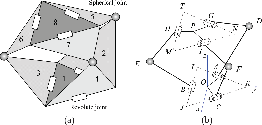
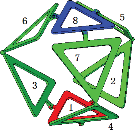
The geometric model and mechanism schematic of the polyhedron robot: (a) geometric model, (b) the mechanism schematic of the robot

(1)

The robot moves by simultaneously actuating the three revolute joints via motors; the rolling motion is achieved when the robot rotates around one of the edges of the base triangle (the triangle that is in contact with the ground).

(2)

In some particular configurations of the robot, we can choose one of six directions to roll along.

(3)

Traditionally, singular positions are avoided for the stability of the mechanism. However, we show how to use the singular positions to realize the capability of rolling and changing directions. This idea is similar to our previous works [21] and [22–23].

(4)

Our robot can be folded into a very compact form. This is convenient for storage and transportation.

2. Mechanism and Kinematics

2.1 Mechanism Design

The geometric model of the robot is shown in Figure 1(a). It resembles a polyhedron; therefore, we call it a polyhedron robot. Each link is an equilateral triangle. These triangles are numbered from 1 to 8, among which 1 and 8 denote the base and top triangles, respectively. The base and top triangle are connected by three chains, each made up of two triangles; in our example, these chains are: 5–2, 6–3, and 7–4. Each chain pair, e.g., 6–3, is connected at a shared vertex via a spherical joint. The upper triangle of the pair is connected to the top, and the lower triangle to the base via revolute joints. Thus, the robot consists of eight links with six revolute joints and three spherical joints. It is a 3-RSR parallel mechanism [24, 25]. The mechanism schematic of the robot is shown in Figure 1(b); links AD, DG, BE, EH, CF and FI represent the triangles 2, 5, 3, 6, 4 and 7, respectively. O and P are the centroids of the base and top, respectively; J, K and L are the vertices of the triangle 1; M, N and T are the vertices of the triangle 8; A, B and C are the midpoints of the edges of triangle 1; H, I and G are the midpoints of the edges of triangle 8.

2.2 Kinematic Analysis

In this mechanism, it is well known that this configuration is non-overconstrained (see, for example, [24] and [25]). Thus, the mobility of our mechanism satisfies the Grübler-Kutzbach mobility condition [26]. Therefore,

M = 6 (n - 1) - \sum_{i = 1}^{g} (6 - f_{i})

(1)

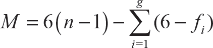
where n is the number of links, g the number of joints, and fi the degree of freedom of the i-th joint. Substituting the parameter values for our robot, M = 6×7 − 39 = 3. The upper triangle 8 will have a translation movement and two rotational movements with respect to the lower triangle 1.

Let θ₁, θ₂ and θ₃ denote the angles between the base triangle and links AD, BE and CF, respectively. We first discuss the ranges of the three angles.

Since all links of the three chains have the same size, according to ref. [24], this polyhedron robot is symmetrical with respect to the plane passing through the three spherical joints, namely the plane DEF. In Figure 2(a), ∠DGP = ∠OAD, ∠EHP = ∠OBE and ∠FIP = ∠OCF. Due to this symmetrical characteristic, as shown in Figure 3, two special positions are obtained. When links AD, BE and CF are all parallel with the lower triangle (i.e., θ₁ = θ₂ = θ₃ = 0), the upper triangle is coincident with the lower one, and the robot is at its lowest position (see Figure 3(a)). Similarly, when links AD, BE and CF are all vertical to the lower triangle (i.e., θ₁ = θ₂ = θ₃ = π/2), the upper triangle is at its highest position (see Figure 3(b)).

Figure 2.

The mechanism schematic of the robot: (a) a common view, (b) a view of the robot where the planes’ DEF, top and base, are projected onto lines

Figure 3.

The limit positions of the upper triangle: (a) the lowest position, (b) the highest position, (c) unstable position

Considering the RSR chain further, if the input angle θ₁ increases from π/2, the links will move inside the mechanism. According to ref. [27, 28, 30], when two or three spherical joints are coincidence, the mechanism is at its singular positions. This can also be identified using the method in ref. [29]. For example, if D and E are coincident, the mechanism will have a free rotation movement about line DF. It is unable to control the mechanism at such singular positions.

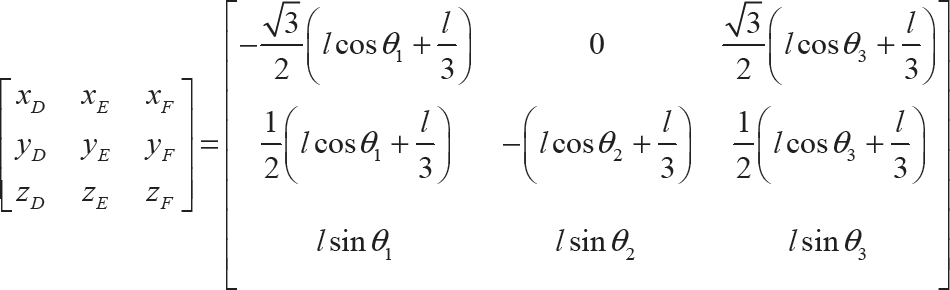
Based on the above discussions, in this paper, we consider that the three angles are in range (0, π/2). Let l be the length of link BE, so the length of OB is l / 3. For any vertex D, we define (xD, yD, ZD)T as the coordinates of D in the coordinate frame with origin at the centroid O of the base, and the y-axis along OK (see Figure 1 (b)). The positions of A, B and C are obtained as

[\begin{matrix} x_{A} & x_{B} & x_{C} \\ y_{A} & y_{B} & y_{C} \\ z_{A} & z_{B} & z_{C} \end{matrix}] = [\begin{matrix} \frac{- \sqrt{3} l}{6} & 0 & \frac{\sqrt{3} l}{6} \\ \frac{l}{6} & \frac{- l}{3} & \frac{l}{6} \\ 0 & 0 & 0 \end{matrix}]

(2)

The positions of D, E and F can be expressed in terms of the values of θ₁, θ₂ and θ₃ by

[\begin{matrix} x_{D} & x_{E} & x_{F} \\ y_{D} & y_{E} & y_{F} \\ z_{D} & z_{E} & z_{F} \end{matrix}] = [\begin{matrix} - \frac{\sqrt{3}}{2} (l \cos θ_{1} + \frac{l}{3}) & 0 & \frac{\sqrt{3}}{2} (l \cos θ_{3} + \frac{l}{3}) \\ \frac{1}{2} (l \cos θ_{1} + \frac{l}{3}) & - (l \cos θ_{2} + \frac{l}{3}) & \frac{1}{2} (l \cos θ_{3} + \frac{l}{3}) \\ l \sin θ_{1} & l \sin θ_{2} & l \sin θ_{3} \end{matrix}]

(3)

Due to the symmetry of the robot, we know that ||DP|| = ||DO||, ||EP|| = ||EO||, and ||FP|| = ||FO||, where ||^*|| denotes the length, and therefore

{\begin{cases} {(x_{P} - x_{D})}^{2} + {(y_{P} - y_{D})}^{2} + {(z_{P} - z_{D})}^{2} = R_{1} \\ {(x_{P} - x_{E})}^{2} + {(y_{P} - y_{E})}^{2} + {(z_{P} - z_{E})}^{2} = R_{2} \\ {(x_{P} - x_{F})}^{2} + {(y_{P} - y_{F})}^{2} + {(z_{P} - z_{F})}^{2} = R_{3} \end{cases}

(4)

where R₁ = ||DO||², R₂ = ||EO||², and R₃ = ||FO||². With some algebraic manipulation, Eq. (4) can be re-written as

{\begin{cases} x_{P} (x_{E} - x_{D}) + y_{P} (y_{E} - y_{D}) + z_{P} (z_{E} - z_{D}) = 0 \\ x_{P} (x_{F} - x_{D}) + y_{P} (y_{F} - y_{D}) + z_{P} (z_{F} - z_{D}) = 0 \end{cases}

(5)

Let $k_{11} = \frac{y_{E} - y_{D}}{x_{E} - x_{D}}$ , $k_{12} = \frac{z_{E} - z_{D}}{x_{E} - x_{D}}$ , $k_{21} = \frac{y_{F} - y_{D}}{x_{F} - x_{D}}$ and $k_{22} = \frac{z_{F} - z_{D}}{x_{F} - x_{D}}$ . Then Eq. (5) can be re-written as

{\begin{cases} x_{P} + k_{11} y_{P} + k_{12} z_{P} = 0 \\ x_{P} + k_{21} y_{P} + k_{22} z_{P} = 0 \end{cases}

(6)

Solving Eq. (6) for (x_p, y_p), we get

{\begin{cases} x_{P} = a_{1} z_{P} \\ y_{P} = a_{2} z_{P} \end{cases}

(7)

where $a_{1} = (- \frac{k_{11} (k_{22} - k_{12})}{k_{11} - k_{21}} - k_{12})$ , $a_{2} = \frac{k_{22} - k_{12}}{k_{11} - k_{21}}$ . With x_p, y_p expressed in Eq. (7), then the first equation of Eq. (4) can be expressed in terms of z_p as

(a_{1}^{2} + a_{2}^{2} + 1) z_{P}^{2} - 2 (a_{1} x_{D} + a_{2} y_{D} + z_{D}) z_{P} = 0

(8)

Solving Eq. (8), we get

{\begin{cases} z_{p} = 0 \\ z_{P} = \frac{2 (a_{1} x_{D} + a_{2} y_{D} + z_{D})}{a_{1}^{2} + a_{2}^{2} + 1} \end{cases}

(9)

When z_P = 0, it means that the upper triangle is coincident with the lower triangle. For a real prototype, this configuration cannot be reached. Thus, we shall ignore the first solution.

It remains to compute the coordinates of G, H, and I. We show how to derive the position of G first; the positions of H and I can be determined similarly. Since the mechanism is symmetrical with respect to the plane DEF, OP is orthogonal to the plane DEF. Thus, the plane DEF is defined by

x_{P} (x - x_{D}) + y_{P} (y - y_{D}) + z_{P} (z - z_{D}) = 0

(10)

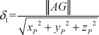
The lines AG, BH, CI and OP are parallel due to the symmetrical structure of the mechanism. So, the parametric equation of the line along AG can be written as A + k1(G – A) = A + k1k₂ (P – O) = A + δ(P), where the bold letters denote the position vectors of the respective points, and δ=k₁k₂. Therefore

{\begin{cases} x = x_{A} + δ x_{P} \\ y = y_{A} + δ y_{P} \\ z = z_{A} + δ z_{P} \end{cases}

(11)

The value of the parameter δ at point G, δ₁, is determined by observing that ||AG|| is twice the distance of point A from the plane DEF, i.e.,

δ_{1} = \frac{‖ A G ‖}{\sqrt{x_{P}^{2} + y_{P}^{2} + z_{P}^{2}}}

(12)

where $‖ A G ‖ = 2 \frac{| x_{P} (x_{A} - x_{D}) + y_{P} (y_{A} - y_{D}) + z_{P} (z_{A} - z_{D}) |}{\sqrt{x_{P}^{2} + y_{P}^{2} + z_{P}^{2}}}$ .

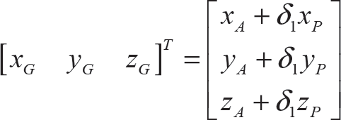
Using Eq. (11) and Eq. (12), the position of Q can be expressed as

{[\begin{matrix} x_{G} & y_{G} & z_{G} \end{matrix}]}^{T} = [\begin{array}{l} x_{A} + δ_{1} x_{P} \\ y_{A} + δ_{1} y_{P} \\ z_{A} + δ_{1} z_{P} \end{array}]

(13)

Similarly, the positions of H and I can be obtained in Eq. (14) and Eq. (15) respectively.

{[\begin{matrix} x_{H} & y_{H} & z_{H} \end{matrix}]}^{T} = [\begin{array}{l} x_{B} + δ_{2} x_{P} \\ y_{B} + δ_{2} y_{P} \\ z_{B} + δ_{2} z_{P} \end{array}]

(14)

where $δ_{2} = 2 \frac{| x_{P} (x_{B} - x_{D}) + y_{P} (y_{B} - y_{D}) + z_{P} (z_{B} - z_{D}) |}{x_{P}^{2} + y_{P}^{2} + z_{P}^{2}}$ .

{[\begin{matrix} x_{I} & y_{I} & z_{I} \end{matrix}]}^{T} = [\begin{array}{l} x_{C} + δ_{3} x_{P} \\ y_{C} + δ_{3} y_{P} \\ z_{C} + δ_{3} z_{P} \end{array}]

(15)

where $δ_{3} = 2 \frac{| x_{P} (x_{C} - x_{D}) + y_{P} (y_{C} - y_{D}) + z_{P} (z_{C} - z_{D}) |}{x_{P}^{2} + y_{P}^{2} + z_{P}^{2}}$ .

2.3 Relationship with Planar Parallelogram Mechanisms

In this section, we will show that in certain configurations of our robot, it is kinematically equivalent to a planar parallelogram mechanism. Furthermore, we perform a numerical verification of the various motion ranges of the mechanism using a commercial solver, MatLab^™.

Consider our robot in Figure 2(a), where the revolute joints corresponding to the input angles θ₁ and θ₃ are locked. Then, the triangles 1, 2 and 4 fuse together into a single link. By symmetry, triangles 8, 5, and 7 also act as a single link. As the input angle θ₂ is changed by a rotation of link BE relative to the base, the two fused links rotate with respect to each other around an axis connecting the centres of the two spherical joints D and F. In other words, the two fused links can be seen as connected with an imaginary revolute joint at the mid-point, Q, of DF. In this configuration, our robot behaves as a four-bar mechanism (BEHQ). Furthermore, for appropriately chosen values of θ₁ and θ₃, we show that it behaves as a planar parallelogram mechanism (PPM). A four-bar mechanism is a PPM if it satisfies the following characteristics:

(1)
The axes of the three revolute joints (here, at B, Q and H) are parallel; and
(2)
The lengths of the opposite links are equal (here, ‖EH‖ = ‖BQ‖ and ‖BE‖ = ‖HQ‖).

To satisfy condition (1), line DF should be parallel with the x-axis. This is true when y_D = y_F and Z_D = Z_F, i.e., θ₁ = θ₃ (using Eq. (3)). Thus, the position of Q can be expressed as

${[\begin{matrix} x_{Q} & y_{Q} & z_{Q} \end{matrix}]}^{T} = {[\begin{matrix} 0 & \frac{l}{2} (\cos θ_{1} + \frac{1}{3}) & l \sin θ_{1} \end{matrix}]}^{T}$
(16)

Then, we get the length of BQ as

$‖ B Q ‖ = \frac{l}{2} \sqrt{{(1+cos θ_{1})}^{2} + 4 \sin^{2} θ_{1}}$
(17)

To satisfy condition (2), we require that ‖BQ‖ = ‖EH‖. Note that ‖EH‖ = ‖BE‖ = l. From Eq. (17), we have

$3 \cos^{2} θ_{1} - 2 \cos θ_{1} - 1 = 0$
(18)

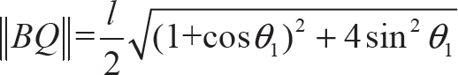
Eq. (18) has a single root at θ₁ = 0. To summarize, when θ₁ = θ₃ = 0, and θ₂ > 0, the mechanism is at its singular position and it becomes a PPM. As shown in Figure 4(a), triangles 1, 2 and 4 and are on the ground and form link BQ, and triangles 8, 5, and 7 are on the same plane and form link HQ. The mechanism becomes PPM BQHE. Similarly, when θ₂ = θ₃ = 0 and θ₁ > 0, we get the PPM ADGR (see Figure 4(b)); when θ₁ = θ₂ = 0 and θ₃ > 0, we get the PPM CFIS (see Figure 4(c)).

Figure 4.
The states when the robot is deformed into a PPM: (a) triangles 1, 2 and 4 are on the ground, (b) triangles 1, 3 and 4 are on the ground, and (c) triangles 1, 2 and 3 are on the ground

Note that each PPM has two assembly modes, e.g., Figure 4(a) shows the first assembly mode of PPM BQHE. Since the lengths of four links are the same, the second assembly mode can be obtained when H and B are coincident. This is a singularity position [27]. However, for the real prototype, this position cannot be reached. We shall consider that the robot can deform into three different PPM states (this is evident from Figure 4, where the dashed blue lines show the equivalent PPM states).

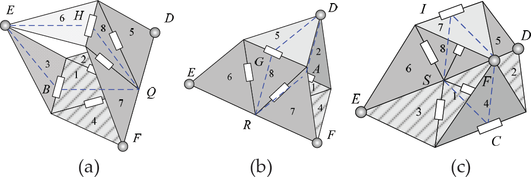
Using Eqs. (1), (2), (7), (9), (13), (14) and (15), the forward kinematics of the robot can be simulated with explicit solutions for the positions of all vertices, given the values for the angles θ₁, θ₂ and θ₃. We implemented this simulation in MatLab^™, setting l = 1 m. The input parameter values corresponding to five positions of interest are shown in the corresponding columns in Table 1. Each of configurations I, II and III correspond to the case in which the device is a PPM. For comparison, we also provide two additional configurations, IV and V, in which the robot is not a PPM. Figure 5 shows plots of the robot corresponding to its PPM configurations.

Figure 5.
Three states of the robot where it is configured as a PPM: (a) configuration I, (b) configuration II, (c) configuration III

Table 1.
Input angles {θ₁, θ₂, θ₃} (rad)

Input angles Config. I Config. II Config. III Config. IV Config. V

θ₁ 0 π/3 0 π/6 π/4

θ₂ π/3 0 0 π/3 π/4

θ₃ 0 0 π/3 π/5 π/4

In Figure 6, we show the planar projections of the configurations when the robot is a PPM. Figure 6(a) shows the view of the robot in configuration I when it is projected onto the BEH plane. Observe that A, B, C, D and F are on a common plane, and H, P, G, I, D and F are on another common plane.

Figure 6.
The projected view of the robot: (a) the projection of configuration I on the BEH plane, (b) the projection of configuration II on the ADG plane, (c) the projection of configuration III on the CFI plane

Using the simulation program, we can also simulate the robot in other configurations when the robot is not a PPM. See Figure 7 for the plots of the robot corresponding to configurations IV and V.

Figure 7.
(a) The robot corresponding to configuration IV in Table 1; (b) the robot corresponding to configuration V in Table 1, where θ₁ = θ₂ = θ₃

Figure 8.
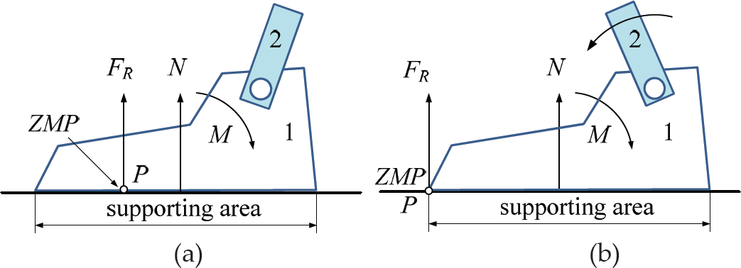
The zero moment point (ZMP) of the robot: (a) ZMP is in the interior of the supporting area, (b) ZMP is on the border of the supporting area
3. Rolling Analysis

Input angles	Config. I	Config. II	Config. III	Config. IV	Config. V
θ₁	0	π/3	0	π/6	π/4
θ₂	π/3	0	0	π/3	π/4
θ₃	0	0	π/3	π/5	π/4

In this section, the feasibility of achieving the rolling motion is analysed, based on the zero moment point (ZMP) analysis of the robot. ZMP is considered the centre of pressure at the feet (supporting area) on the ground. As shown in Figure 8, link 1 is a supporting foot, and link 2 is connected to link 1 via a revolute joint. The ground reaction force can be viewed as a force N and the torque M at the centre of the supporting area. Consider a point P on the ground, such that the sum of the forces at it is F_R; if the torque at P caused by F_R; is zero, then P is called the zero moment point (ZMP) of the robot [31]. In Figure 8(a), P is in the interior of the supporting area and the robot is in a state of dynamic balance. As the link 2 rotates counter-clockwise, P moves to the left; at some stage, if P coincides with the left endpoint of the supporting area (see Figure 8(b)), then the robot is about to lose its dynamic balance and can rotate about the left endpoint [32].

Without loss of generality, assume that our robot is rolling along the positive y-axis (see Figure 9). It is then sufficient to consider the projection of the ZMP on the y-axis since the robot is planar. We denote this component by y_zmp. Using an analysis similar to those of Takanishi [33] and Kim [34], y_zmp can be expressed as follows:

Figure 9.

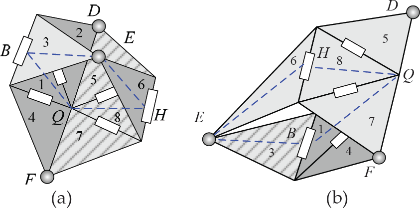
The schematic of the PPM: (a) the state when triangles 1, 2 and 4 are on the ground, (b) the simplified sketch of the PPM

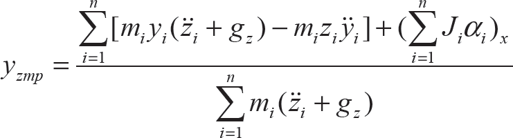
y_{z m p} = \frac{\sum_{i = 1}^{n} [m_{i} y_{i} ({\ddot{z}}_{i} + g_{z}) - m_{i} z_{i} {\ddot{y}}_{i}] + {(\sum_{i = 1}^{n} J_{i} α_{i})}_{x}}{\sum_{i = 1}^{n} m_{i} ({\ddot{z}}_{i} + g_{z})}

(19)

where m_i is the mass of link i, x_i, y_i and z_i are the accelerations along the x-axis, y-axis and z-axis respectively, g_z is the acceleration due to gravity, P_i = (x_i y_i z_i)^T is the centre of mass of link i, α_i is the angular acceleration of link i, and (J_iα_i)_x is the moment of inertia about the x-axis of link i. When y_zmp moves out of the supporting area, the robot will rotate about the corresponding triangle edge, executing a tumbling motion.

As shown in Figure 9, link BQ lies along the positive y-axis. Link BE and link EH have the same mass, and link BQ and link QH have the same mass. Let m1 and m2 be the mass of the links BE and BQ respectively. Let ω and α be the angular velocity and acceleration of link BE, respectively.

The centre of mass of each link P_i can be computed from Eq. (20). Deriving the second derivative of each P_i, the accelerations along the x-axis, the y-axis and the z-axis of each P_i are expressed in Eq. (21). Based on the schematic of the robot in Figure 9(b), the moment of inertia about the x-axis of each link is shown in Eq. (22).

[\begin{matrix} P_{1} \\ P_{2} \\ P_{3} \\ P_{4} \end{matrix}] = [\begin{matrix} 0 & \frac{l \cos θ}{2} & \frac{l \sin θ}{2} \\ 0 & l (\frac{1}{2} + \cos θ) & l \sin θ \\ 0 & l (1 + \frac{\cos θ}{2}) & \frac{l \sin θ}{2} \\ 0 & \frac{l}{2} & 0 \end{matrix}]

(20)

[\begin{matrix} {\ddot{P}}_{1} \\ {\ddot{P}}_{2} \\ {\ddot{P}}_{3} \\ {\ddot{P}}_{4} \end{matrix}] = [\begin{matrix} 0 & u & v \\ 0 & 2 u & 2 v \\ 0 & u & v \\ 0 & 0 & 0 \end{matrix}]

(21)

where u = 0.5l(–αsingθ – ω² cos θ) v = 0.5l(α cos θ – ω² sin θ).

[\begin{matrix} {(J_{1} α_{1})}_{x} & {(J_{2} α_{2})}_{x} & {(J_{3} α_{3})}_{x} & {(J_{4} α_{4})}_{x} \end{matrix}] = [\begin{matrix} \frac{m_{1} l α}{12} & 0 & \frac{m_{1} l α}{12} & 0 \end{matrix}]

(22)

Substituting Eqs. (20)-(22) into Eq. (19), the y_zmp can be expressed as

y_{z m p} = \frac{K_{1} u + K_{2} v + K_{3}}{4 g (m_{1} + m_{2}) + (6 m_{1} + 2 m_{2}) v}

(23)

where $\begin{array}{l} K_{1} = l \sin θ (- 5 m_{1} - m_{2}) \\ K_{2} = l (2 m_{1} + 2 m_{2} + 5 m_{1} \cos θ + m_{2} \cos θ) \\ K_{3} = g l (m_{1} + 3 m_{2} + 3 m_{1} \cos θ + m_{2} \cos θ) + \frac{m_{1} l α}{3} \end{array}$ .

For the PPM shown in Figure 9, the supporting area along the y-axis is [0, l]. As y_zmp moves out of the supporting area, the robot will tumble. Therefore, the rolling condition can be expressed as

{\begin{cases} y_{z m p} = \frac{K_{1} u + K_{2} v + K_{3}}{4 g (m_{1} + m_{2}) + (6 m_{1} + 2 m_{2}) v} > l \\ y_{z m p} = \frac{K_{1} u + K_{2} v + K_{3}}{4 g (m_{1} + m_{2}) + (6 m_{1} + 2 m_{2}) v} < 0 \end{cases}

(24)

We now look at a simple numerical example to illustrate the use of this formulation. Suppose that the initial parameters of the robot are assigned as follows: l = 1 m, m1 = 1 kg, m2 = 3 kg. Assume that the robot starts from an initial position as shown in Figure 9(b). At this moment, BQ and BE are parallel to the y-axis and z-axis, respectively, i.e., θ = π/2. We define ωas positive when link BE rotates counter-clockwise around point B. When ω < 0, as θ is decreasing, the PPM will move to the right with its supporting area along the y-axis on the interval [0, 1]. If y_zmp moves outside this range, then the robot will roll.

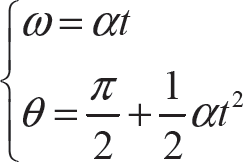
Suppose that, at the initial state (π/2), the initial angular velocity equals to zero, and the motor starts with a constant angular acceleration α. After time (t), we can use the following equations to obtain the angular velocity and the displacement of θ.

{\begin{cases} ω = α t \\ θ = \frac{π}{2} + \frac{1}{2} α t^{2} \end{cases}

(25)

As the robot deforms, the yzmp will move out of its supporting area. Depending on whether α > 0, we have the following two cases.

Case 1: α < 0, link BE is accelerating to the right.

To illustrate the effects of α on yzmp, suppose we choose α = {-1, −1.5, −2} rad/s². Once yzmp moves out of the upper limit of the equilibrium position, the robot begins to roll to the right. As shown in Figure 10, when α = −1 rad/s², yzmp is out of the upper limit of the equilibrium position when θ≈ 0.377 rad (the solid line). Further, according to Eq. (25), the angular velocity at this moment is 1.545 rad/s. Likewise, when α = −2.0rad/s², yzmp will be out of the equilibrium range when θ≈ 0.574 rad (the dotted line), and the angular velocity is 1.999 rad/s. From the trends of the curves, we can also see that the robot can roll to the right more easily as α increases, which is also intuitive. We shall stop the motor immediately during this rolling process, so that the angular velocity will be decreased to zero in a very short time.

Figure 10.

The curves of yzmp when the robot rolls to the right

Case 2: α > 0, link BE is accelerating to the left.

Let α = {1, 1.5, 2}rad/s². As shown in Figure 11, when α < 9.2 rad/s², yzmp is not out of the lower limit of the equilibrium position, and the robot cannot roll during the motion. When α≈ 9.2 rad/s², yzmp will be out of the equilibrium range when θ≈ 2.53 rad (the dashed line), and the angular velocity is 4.201 rad/s. From the trends of the curves, we can also see that the robot can roll to the right more easily as α increases, which is also intuitive. This is due to the difference in the weights of the links.

Figure 11.

The curves of yzmp when the robot rolls to the left

4. Direction switching function

In this section, we discuss the rolling direction of the robot. Referring to the initial configuration in Figure 9, when triangle 1 is supported on the ground, we have three different states of PPM. Each PPM has its own directions. By switching between these states, the robot can choose its moving direction. Recall that O is the centre of triangle 1. As shown in Figure 12, the robot can choose any one of six directions (dashed arrows) to move along when triangle 1 is on the ground. A similar choice is available when triangle 8 is on the ground.

Figure 12.

The six directions the robot can choose to move in

According to the analysis in section 3, it is possible to make the robot roll along either the positive or negative y-axis. If the robot rolls to the positive y-axis, then link QH (i.e., triangle 8) becomes the new supporting area, the resulting state of the robot is shown in Figure 13(a). As pointed out above, the robot can also choose one out of six directions to roll along in the next stage. However, if it rolls to the negative y-axis, then link BE becomes the new supporting area; the resulting state of the robot is shown in Figure 13(b). From this position, the robot can only choose to move forwards or backwards along line BE, by rotating the revolute joint at B, i.e., changing θ₂.

Figure 13.

(a) The state when triangles 5, 7 and 8 are on the ground, (b) the state when triangle 3 is on the ground

In summary, with two motors being locked, the robot can roll with one DOF. At the same time, since the DOFs of the robot are three, we can use this flexibility to provide a direction switching functionality, which can be useful in moving around obstacles.

5. Simulation

The kinematic feasibility of the designed robot is tested by generating a simplified solid model using SolidEdge^™ (Figure 14), and then simulating the motion by specifying the appropriate constraints at each joint in ADAMS^™.

Figure 14.

The simulation model of the robot (a common state)

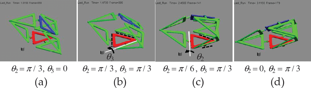
Let the configurations of the robot in Figure 4(a), (b) and (c) be denoted as State A, State B and State C, respectively. Considering Figure 15 (the white dashed line denotes the active joint, while the black dashed line denotes the locked joints), we can switch from State A to State B by first rotating triangle 2 by increasing θ₁ to π/3, and then rotating triangle 3 by decreasing θ₃ from π/3 to 0.

Figure 15.

Simulated motion of the robot as it switches from State A to State B. The base (red) and top (blue) triangles are shown in different colours for clarity (the position of the bulk is fixed on the ground)

It is easy to show that, in a similar fashion, the robot can switch from any of the three states to an alternate one (e.g., to go from State A to State C, first rotate triangle 4 by increasing θ₃ to π/3 and then rotate triangle 3 by decreasing θ₂ to 0); similar transitions can be achieved when the top face (face 8) is resting on the ground. Figure 16 shows a few positions during the switch from State A to State C (the white dashed line denotes the active joint, while the black dashed line denotes the locked joints). Figure 17 illustrates a rolling simulation process when the robot is in State A.

Figure 16.

Simulated motion of the robot as it switches from State A to State C. The base (red) and top (blue) triangles are shown in different colours for clarity (the position of the bulk is fixed on the ground)

Figure 17.

A rolling simulation when the robot is in State A

From the simulation procedure, it is shown that the direction switching function can be realized by manipulating two motors, while the rolling function is realized by operating a single motor; i.e., the robot realizes the direction switching function and the rolling function with two DOFs and one DOF, respectively.

6. Prototype and Experiment

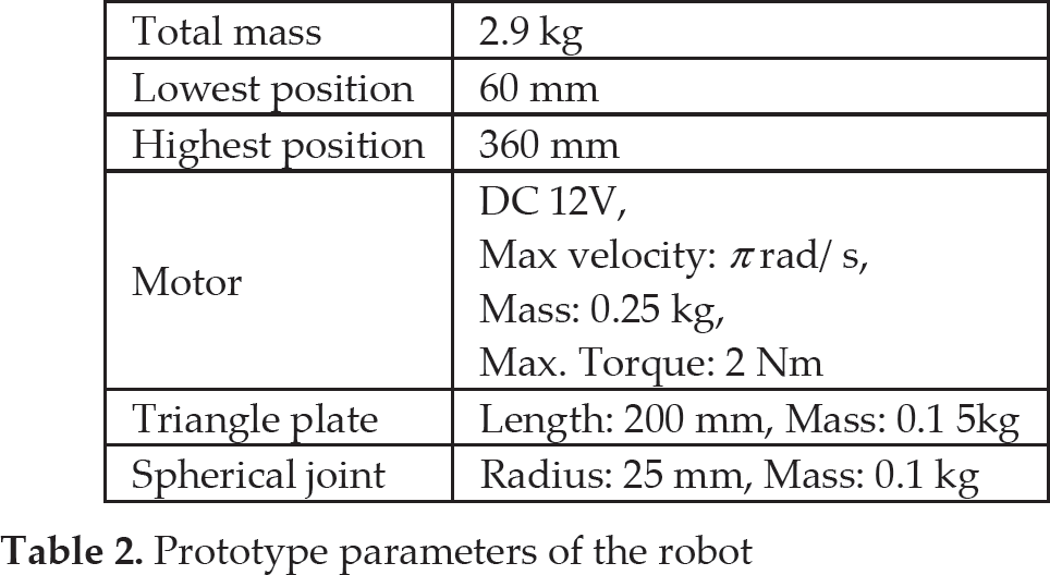
A prototype was fabricated to test the performance of the designed robot (see Figure 18). The major parameters of our robot are shown in Table 2. Note that the robot can be driven by three motors, with a motor being installed at the end of each chain. However, to balance the weight of the robot and to efficiently control the rolling directions, our design includes two working motors on both ends of each chain.

Figure 18.

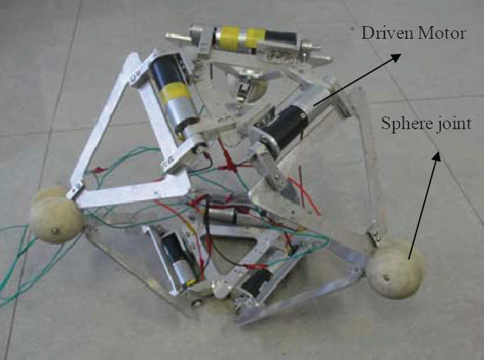
The prototype of the robot

Figure 19 shows the folding function of the robot. Figure 20(a)–(c) shows the prototype in States A, B and C, respectively, and the dashed lines denote the rolling directions. Figure 21 shows a rolling process when the robot is in State A.

Figure 19.

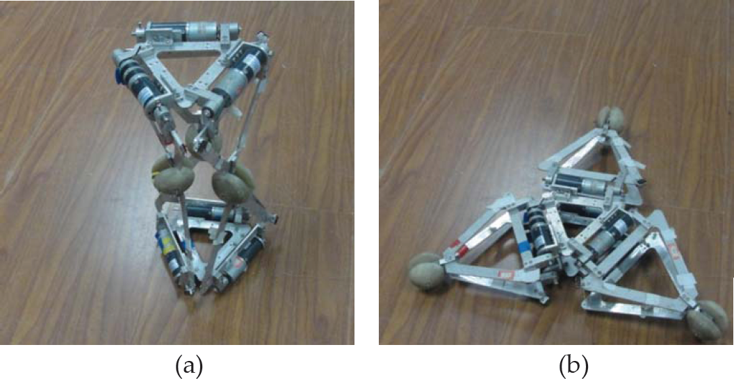
The robot can be folded from its tallest status (a) to an extremely compact form (b)

Figure 20.

States of the prototype robot corresponding to State A, B and C in Figure 4

Figure 21.

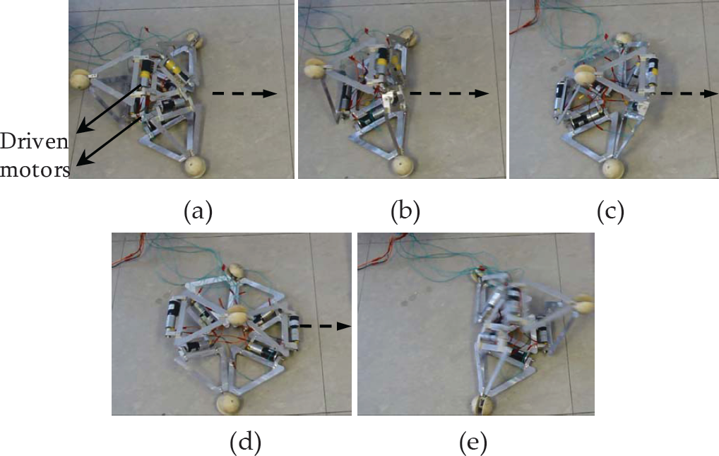
Illustration of the rolling function (the dashed lines denote the rolling direction)

Table 2.

Prototype parameters of the robot

Total mass	2.9 kg
Lowest position	60 mm
Highest position	360 mm
Motor	DC 12V, Max velocity: πrad/ s, Mass: 0.25 kg, Max. Torque: 2 Nm
Triangle plate	Length: 200 mm, Mass: 0.1 5kg
Spherical joint	Radius: 25 mm, Mass: 0.1 kg

7. Conclusions

In this paper, a new rolling robot is introduced. It can switch rolling directions at its singular positions, and it can be folded into a very compact form. We analysed the kinematics of the robot. We demonstrated how the robot can achieve two types of motions: a linear rolling motion and a reconfiguration motion that allows the robot to change its moving directions. The rolling conditions are computed based on a ZMP analysis, and can potentially be used for velocity/acceleration control. A CAD-based assembly model was used to verify the mobility of the robot. Finally, a physical prototype was constructed to demonstrate the ability of the robot to achieve the motion modes described in this paper.

The focus of this paper is to introduce and analyse the motion of this new rolling robot. In our future work, we are going to improve this robot in two ways. Firstly, the kinematics can be further analysed considering all the singularity positions. Based on the kinematics, the rolling gaits on uneven ground can also be studied. Secondly, we are going to improve the prototype for future tests in realistic situations. This might include, for example, deploying on-board batteries for powering the motors, adding servo-controls to the motors, and possibly adding an on-board vision system to identify obstacles and perform real-time adaptive path planning.

8. Acknowledgements

This work has been supported by the National Natural Science Foundation of China (51175030), and Fundamental Research Funds for the Central Universities (2011JBM277 and 2012JBZ002). Part of the work in this paper was funded by GRF grant #614205.

References

Machado

J. A. T.

and Silva

M. F.

(2006) An overview of legged robots. International Symposium on Mathematical Methods in Engineering. Ankara, Turkey, MME Press.

Cobano

J. A.

Estremera

and Santos

P. G.

(2008) Location of legged robots in outdoor environments. Robot. Auton. Syst., 56(3): 751–761.

Battaglia

Cocosco

Hawker

Sarkis

and Yamazaki

(1998) SCOUT: A simple quadruped that walks, climbs, and runs. Proc. IEEE ICRA, Belgium, pp. 1701–1712.

Poulakakis

Smith

J. A.

and Buehler

(2004) Experimentally validated bounding models for the Scout II quadrupedal robot. Proc. IEEE ICRA, Louisiana, pp. 2595–2600.

Smith

J. A.

and Poulakakis

(2004) Rotary gallop in the untethered quadrupedal robot Scout II. Proc. IEEE/RSJ Int. Conf. IROS, Sendai, pp. 2556–2561.

Raibert

Blankespoor

Nelson

and Playter

(2008) Bigdog, the rough-terrain quadruped robot. Int. Conf. Automatic Control World Congress, Seoul, pp. 10822–10825

Raibert

M. H.

(1986) Legged robots that balance. Cambridge, Mass., MIT Press.

Hirose

(1993) Biologically inspired robots: Snake-like locomotors and manipulators. Oxford, Oxford University Press.

Chernousko

F. L.

and Shunderyuk

M. M.

(2010) The influence of friction forces on the dynamics of a two-link mobile robot. J. Appl. Math. Mech., 74(1): 13–23.

10.

Yim

Homans

and Roufas

(2001) Climbing with snake-like robots. Proc. IFAC. Workshop on Mobile Robot Technology, Jejudo, Korea, pp. 21–22.

11.

Araya

and Li

(2001) Development of a creeping snake-robot. Proc. IEEE Int. Symposium on Computational Intelligence in Robotics and Automation, Banff, Alberta, Canada, pp. 77–82.

12.

Armour

R. H.

and Vincent

J. F. V.

(2006) Rolling in nature and robotics: a review. J. Bionic Eng., 3:195–208.

13.

Bhattacharya

and Agrawal

S.K.

(2000) Spherical rolling robot: A design and motion planning studies. IEEE T. Robot. Autom., 16(6): 835–839.

14.

Javadi

A. H.

and Mojabi

(2004) Introducing glory: A novel strategy for an omnidirectional spherical rolling robot. ASME J. Dyn. Syst-T., 126(3): 678–683.

15.

Das

and Mukherjee

(2004) Exponential stabilization of the rolling sphere. Automatica, 40(11): 1877–1889.

16.

Joshia

V. A.

and Banavar

R. N.

(2009) Motion analysis of a spherical mobile robot. Robotica, 27: 343–353.

17.

Joshia

V. A.

Banavar

R. N.

and Hippalgaonkar

(2010) Design and analysis of a spherical mobile robot. Mech. Mach. Theory, 45(2): 130–136.

18.

Sastra

Chitta

and Yim

(2009) Dynamic rolling for a modular loop robot. Int. J. Robot. Res., 28(6): 758–773.

19.

Lee

W. H.

and Sanderson

A. C.

(2002) Dynamic rolling locomotion and control of modular robots. IEEE T. Robotic. Autom., 18(1): 32–41.

20.

Clark

P. E.

Rilee

M. L.

Curtis

S. A.

Truszkowski

Marr

Cheung

and Rudisill

(2004) BEES for ANTS: Space mission applications for the autonomous nanotechnology swarm. AIAA 1st Intelligent Systems Technical Conference, Abrahantes.

21.

Liu

and Yao

Y-A.

(2009) Biped RCCR robot. ASME, J. Mech. Des. 131 (3): 031010.1–031010.6.

22.

Liu

Yang

H. H.

and Yao

Y-A

(2012) A family of biped mechanisms with two revolute and two cylindric joints. ASME, J. Mech. Robot. 4(4), 045002–1–045002–13.

23.

Tian

Y.B.

Wei

X. Z.

Joneja

and Yao

Y-A.

(2014) Sliding-crawling parallelogram mechanism. Mech. Mach. Theory, 78, 201–228.

24.

Dunlop

D. R.

and Jones

T. P.

(1997) Position analysis of a 3–DOF parallel manipulator. Mech. Mach. Theory, 32(8): 903–920.

25.

Karouia

and Hervé

J. M.

(2005) Asymmetrical 3-dof spherical parallel robots. Eur. J. Mech. A-Solid, 24(1): 47–57.

26.

Gogu

(2005) Mobility of robots: a critical review. Mech. Mach. Theory, 40(9): 1068–1097.

27.

Gosselin

and Angeles

(1990), Singularity analysis of closed-loop kinematic. IEEE T. Robotic. Autom. 6(3): 280–290.

28.

Pashkevich

Chablat

and Wenger

(2006). Kinematics and workspace analysis of a three-axis parallel manipulator: The Orthoglide. Robotica, 24: 39–49.

29.

Kong

and Johnson

, (2014) Classification of screw systems composed of three planar pencils of lines for singularity analysis of parallel mechanisms, ASME J. Mech. Rob., 6(2): 021008–1–10.

30.

Yang

Chen

I. M.

Lin

, and Angeles

, (2001) Singularity analysis of three-legged parallel robots based on passive joint velocities, Trans. Rob. Autom., 17(4): 413–422.

31.

Vukobratović

Frank

A. A.

and Juricic

(1970) On the stability of biped locomotion. IEEE J. Biomed. Eng., 17(1): 25–36.

32.

Vukobratović

and Borovac

(2008) Dynamic balance concept and the maintenance of the dynamic balance in humanoid robotics. IEEE 6th Intelligent Systems and Informatics, Belgrade, pp. 1–11.

33.

Takanishi

Tochizawa

Takeya

Karaki

and Kato

(1989) Realization of dynamic biped walking stabilized with trunk motion under known external force. Proc. Int. Conf. Advanced Robotics, Columbus, pp. 323–330.

34.

Kim

Chung

W. K.

Youm

and Lee

B. H.

(2002) Real-time ZMP compensation method using null motion for mobile manipulators. Proceedings of IEEE International Conference on Robotics and Automation, Washington, DC, pp. 1967–1972.

Design and Rolling Analysis of a Novel Deformable Polyhedron Robot

Abstract

Keywords

1. Introduction

2.1 Mechanism Design

2.2 Kinematic Analysis

8. Acknowledgements

References