
Abstract
This paper introduces an adaptive backstepping control law for a two-wheel electric scooter (eScooter) with a nonlinear uncertain model. Adaptive backstepping control is integrated with feedback control that satisfies Lyapunov stability. By using the recursive structure to find the controlled function and estimate uncertain parameters, an adaptive backstepping method allows us to build a feedback control law that efficiently controls a self-balancing controller of the eScooter. Additionally, a controller area network (CAN bus) with high reliability is applied for communicating between the modules of the eScooter. Simulation and experimental results demonstrate the robustness and good performance of the proposed adaptive backstepping control.
Keywords
Introduction
A self-balancing two-wheel electric scooter (or eScooter) based on an inverted pendulum model [1–3] is a highly nonlinear system with uncertain parameters, which is very difficult to control with six variable state parameters. Up to now, some research results published on self-balancing two-wheeled mobile robots have focused on the following issues. Papers [4–5] presented the development of two-wheeled mobile robots (TWMRs). TWMRs, such as the selection of actuators and sensors, signal processing units, modelling and the control scheme were addressed and discussed. In addition, the TWMRs were tested using the pole-placement method. Shui Chun Lin et al. [6] introduced a self-balancing human transportation vehicle for teaching the feedback control concept, such as pole-placement control and PID control. Takei et al. [7] introduced linear quadratic regulation (LQR) for a self-balancing controller. However, these methods can only work well when the eScooter is approximately linear at small tilt angles, and where the eScooter's parameters are constant.
Wu et al. [8] and Yau et al. [9] introduced the modelling of TWMRs and the design of sliding mode control for the system. A robust controller based on sliding mode control was proposed to perform the robust stabilization and disturbance rejection of the system. The simulation results were carried out to access the performance of the proposed control law. However, due to switching around the sliding surface, there could be significant chattering.
Backstepping control as a technique was developed in 1990 by Petar V. Kokotovic [10] for the design of stable control applied to a special class of nonlinear dynamic systems. A backstepping control method based on the Lyapunov design approach was efficiently applied when there was a higher derivative appearance in a parametric estimation process. The papers [11–12] introduced the backstepping control used for two-wheeled mobile robot motion. However, conventional backstepping control needs accurate model parameters. Tsai et al. [13] introduced combining backstepping control with a sliding mode control approach for TWMRs. The simulation results demonstrated that the chattering feature was suppressed with the proposed control. However, due to a change in the height of the centre of gravity, various adaptive control strategies should have been used.
Kausar et al. [14] introduced TWMRs able to avoid the tip-over problem on inclined terrain by adjusting the centre of mass position of the robot body. The paper introduced a full state feedback controller based on the LQR method with speed tracking on horizontal flat terrain. The performance and stability regions were simulated for the robot on horizontal flat and inclined terrain with the same controller. The results endorse a variation in the equilibrium point and a reduction in the stability region for robot motion on inclined terrain.
Park et al. [15] proposed an adaptive neural sliding mode control method for the trajectory tracking of a nonholonomic wheeled mobile robot with model uncertainties and external disturbances. Self-recurrent wavelet neural networks (SRWNNs) were used for approximating arbitrary model uncertainties and external disturbances. The simulation results demonstrated the robustness and performance of the proposed control system. Tsai et al. [16] presented an adaptive control using radial basis function neural networks (RBFNNs) for a two-wheeled self-balancing scooter. The proposed two adaptive controllers using RBFNNs were optimized by a backpropagation algorithm to achieve self-balancing and yaw control. However, a neural network control needs considerable training time, a large amount of memory and they sometimes fall into a local optimum.
In this paper, an adaptive backstepping control for an eScooter is proposed and validated. The key idea behind adaptive backstepping control is to converge the error equation to zero by designing a Lyapunov stability approach [17–18]. By using the recursive structure to find the controlled function and then estimate the uncertain parameters, an adaptive backstepping control induces a feedback control law that ensures the efficient control of the eScooter model.
The eScooter consists of two coaxial wheels which are mounted parallel to each other and operated by two brushless DC electric motors (BLDC motors). An accelerometer and gyro sensor are used to measure the pitch angle of the eScooter. In addition, a potentiometer is used to measure the yaw angle of the eScooter. Furthermore, a controller area network (CAN bus) is applied for communicating among the controlling and display modules of the eScooter. In this way, the eScooter can carry the human load up to 85 kg.
The rest of this paper is organized as follows. Section 2 describes the mathematical model of the proposed eScooter. Section 3 introduces an adaptive backstepping control design and then presents simulation results. Section 4 introduces the hardware setup and signal processing using a Kalman filter. Section 5 presents some experimental results. Finally, some conclusions are presented in Section 6.
Mathematical Model of the eScooter
In this section, the Newton method is applied for determining the mathematical model of the eScooter [4–5]. Figure 1 shows the coordinate system of the eScooter.
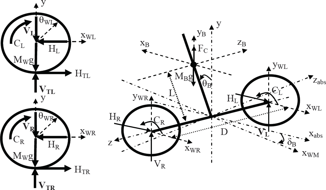
Coordinate system of the eScooter
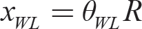
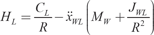
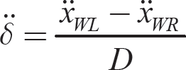
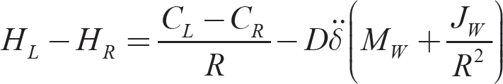
For the left wheel of the eScooter (the same as the right wheel):


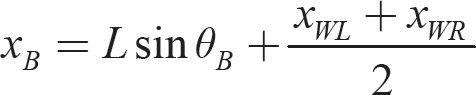
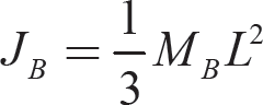
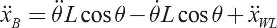
For the body of the eScooter:


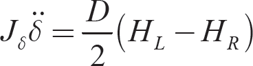
where H
Parameters of the eScooter

Substituting (7), (8) and (13) into (9), we obtain:

From (10), (11) and (14), we infer:

Substituting (17) and (12) into (16), we obtain:

Where, Cθ =CL + CR
From (1), we infer:

Substituting (3) and (7) into (19), we obtain:

From (10) and (14), we derive:
Substituting (21) and (5) into (20), we obtain:

Solving the system of equations (18) and (22), we obtain:


On the other hand, from (1), (3) and (4) we have:
From (6), we get:
Substituting (27) into (15), we obtain:
We have:

Substituting (29) into (28), we obtain:
In summary, the state-space equations of the eScooter are described by (23), (24) and (30), where:

In this section, we introduce the development of the control system for the eScooter. The general structure of the proposed eScooter controller is illustrated in Figure 2.

Block diagram of the proposed eScooter controller
The main features of the proposed eScooter controller are depicted as follows:
A self-balancing controller is used to control the eScooter in equilibrium with a pitch angle θ = 0°. In this paper, adaptive backstepping control is applied to design a self-balancing controller for the eScooter.
A left- and right-turning controller is designed to control the eScooter in turning left and right. In this paper, a PD control is used to design a left- and right-turning controller for the eScooter.
First, the state variables are defined as x1 = θ,

Where:
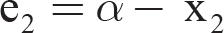
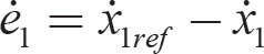
The error equation is defined as:

where θref, which is the referential value of the pitch angle signal θ, is equal to zero for the proposed eScooter self-balancing controller.

where k1 and c1 are positive constants and
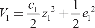
The first Lyapunov function is declared and defined as:
Differentiating (35), we obtain:

Substituting (37) and (34) into (31), we obtain:

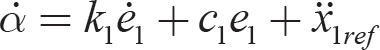
By using the derivative of e2 to ensure the desired dynamic feature for the velocity tracking error. We get:

Differentiating (33) and (34) we obtain:
Substituting (41), (40), (38) and (32) into (39), we obtain:

Substituting (40) and (38) into (36), we obtain:

Continually, the second Lyapunov function is declared and defined as:
Substituting (43) into and differentiating (44), we obtain:

For

where k2 is a positive constant.
Substituting (46) into (45), we obtain:

From (46), we derive:

From (48) and (42), the control signal Cθ is determined as:

where:


In this case, the second error e2 (42) is rewritten as:

On the other hand, we have:
Call

Substituting (54) into (52), we obtain:

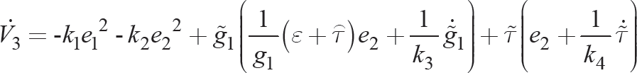
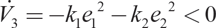
Now, the adaptive laws can be constructed by using the Lyapunov energy function V3 which is defined as:

where k3 and k4 are positive constants.
Differentiating (56), we obtain:

Substituting (55) and (45) into (57), we obtain:
The adaptive laws are implemented as follows:
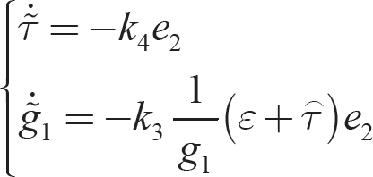
Then, the equation (58) is rewritten as:
with
Finally, the control signal function Cθa is determined as:

In summary, an adaptive backstepping control has been successfully designed. Based on equation (61), we see that the control signal Cθa does not depend on the uncertainty parameters and perturbation of the eScooter.
The general structure of the left- and right-turning controller is depicted in Figure 3.

Left- and right-turning controller block diagram
The main features of the left- and right-turning controller are described as follows:
The reference signal δ ref = 0
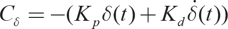
The PD controller is depicted as Gc (s) = Kp + Kds
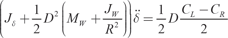
Using (30), the transfer function of the eScooter is determined:

The transfer function describes the overall system:

For closed-loop system stability, it needs:

where ∊ is the damping ratio and ω n represents the natural frequency.
From (64), we derive
Combining the self-balancing controller with the left- and right-turning controller, we obtain the eScooter controller design. The scheme is depicted in Figure 4.

Input torque applied for the right and left wheels
Simulation tests were executed using the eScooter's parameters as tabulated in Table 1. The adaptive backstepping controller parameters are selected as k1 = 15, k2 = 26.4, c1 = 0.001, c4 = 0.001, c5 = −0.95 and the PD controller values selected as ∊ = 1,ω n = 10. Figure 5 illustrates the block diagram of the proposed controller for the eScooter. Figure 6 is the block diagram of the adaptive backstepping controller. These diagrams are executed in the MATLAB/Simulink environment.
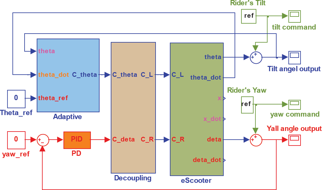
Block diagram of the proposed controller for the eScooter

Block diagram of the adaptive backstepping control
Figure 7 shows the simulation results of the eScooter pitch angle and torque output of the adaptive control Cθ. We see that these values converge on zero from an initial 0.1 radian value. Figure 8 represents the convergence of the unknown g1 and τ parameters, respectively. Similarly, Figure 9 illustrates the simulation results of the eScooter pitch angle and torque output of the adaptive control Cθ. We see that these values quickly converge on zero from an initial −0.15 radian value. Figure 10 represents the convergence of the unknown g1 and τ parameters, respectively.

eScooter tilt angle response with an initial 0.1 radian

Convergence of the unknown g1 and τ parameters with an initial 0.1 radians

eScooter tilt angle response with an initial −0.15 radians.

Convergence of unknown g1 and τ parameters with an initial −0.15 radians
Figure 11 shows the simulation results of the eScooter yaw angle response. These good results, which were collected from three cases of PD controller parameters, are selected as ∊ = 0.5, ω n = 10; ∊ = 1, ω n = 10; or ∊ = 2, ω n = 10, respectively.
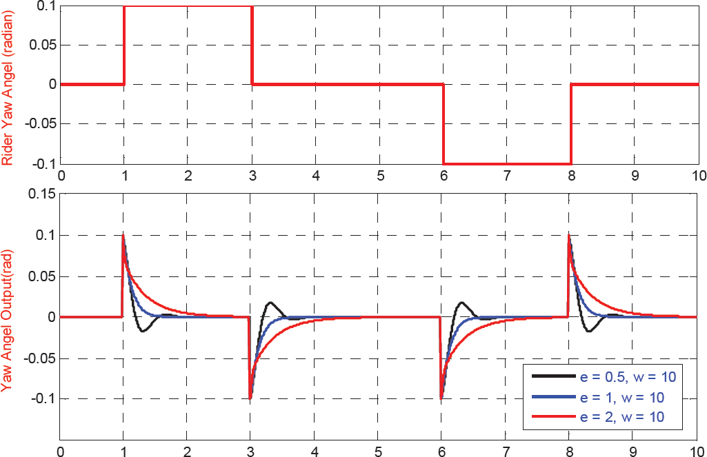
eScooter yaw angle response from three cases of PD controller parameters
Figure 12 shows the simulation results of the eScooter with the pitch and yaw angle responses, the input torque applied for the right and left wheels (CR and CL), the convergence of unknown g1 and τ parameters. Based on Figure 4, the input torque CL and CR are determined and saturated to suitable for characteristics of BLDC motor. We see that eScooter is efficiently controlled through rider's tilt angle and rider's yaw angle.
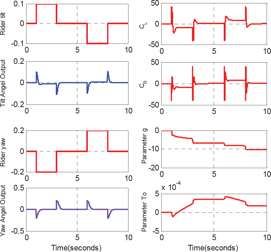
eScooter is controlled through the rider's tilt angle and yaw angle
Based on these results, the proposed control algorithm combining the adaptive backstepping control based on Lyapunov theory and the PD control effectively exhibits robustness in the presence of uncertainty parameters and disturbances for tracking problems.
Hardware Descriptions
The main characteristic of the proposed eScooter is its self-balancing capability. This feature helps the eScooter to always stay in equilibrium, despite the eScooter being equipped with only one axis with two wheels. The driver commands the eScooter to go forwards by shifting their body forwards on the platform, and to go backwards by shifting their body backwards. Furthermore, in order to turn, the driver needs to guide the handlebar to the left or the right. To execute this feature, the hardware of the eScooter is designed as follows. The eScooter is made of two coaxial wheels which are mounted parallel to each other and are driven by two brushless DC electric motors (BLDC motors). Figure 13 shows the block diagram of the eScooter control architecture.

Block diagram of the control architecture of the eScooter
An accelerometer and gyro sensors are used for measuring the pitch angle of eScooter. The potentiometer is used for measuring the yaw angle of the eScooter. These signals are measured by an ADC (analogue-to-digital converter) of the master module that is implemented on an embedded dsPIC board. The data are filtered by a Kalman filter before providing for the self-balancing and turn left-right controller. The eScooter includes three slave modules which are implemented on an embedded dsPIC board. Concretely, slave modules one and two control the left and right wheels of the eScooter, respectively. Slave module three (HMI) displays the eScooter's speed via a graphic screen.
The CAN (controller area network) bus is applied for communicating between the master module with other slave modules, as illustrated in Figure 14. This is due to certain advantages, such as a transfer speed up to 1MB, high reliability and good flexibility. The CAN bus helps us to control the eScooter hierarchy and satisfies the requirements of the real-time operation of the eScooter.

CAN bus architecture in the eScooter
Thanks to these good features, the eScooter can carry a human load of up to 85 kg. Figure 15 shows a photograph of the eScooter.
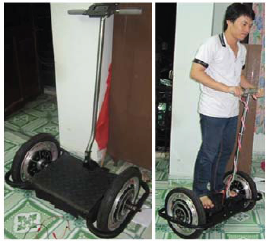
The photograph of the eScooter
The Kalman filter estimates a process by using a form of feedback control [19]. The filter estimates the process state at a given time and then obtains feedback in the form of (noisy) measurements. The equations for the Kalman filter fall into two groups: time update equations and measurement update equations, are illustrated as Figure 16.
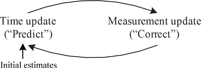
The discrete Kalman filter cycle
The time update equations (66) and (67) are responsible for projecting forward the current state and error covariance estimates to obtain the estimates for the next time step:


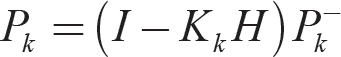
The measurement update equations (68), (69) and (70) use the current measurements to improve the estimates which are obtained from the time-update equations:


The parameters of the discrete Kalman filter used for signal processing from the accelerometer and gyro sensors’ signal are determined as follows:

After signal processing using the discrete Kalman filter, the pitch angle of the eScooter is better than the unfiltered angle measurement, as shown as Figure 17.
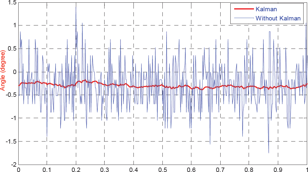
Sensor noise filtering result using a Kalman filter
After embedding the signal processing and control algorithm into the eScooter's hardware, the eScooter gave good performance not only in terms of backwards and forwards movement, but also in turning left and turning right. Figure 18 proves that the pitch angle response oscillates around the equilibrium value 0° when the eScooter has no effect on the outside force.

The response of the pitch angle at the equilibrium
Figure 19 shows that the pitch angle response only sways for around 0.7 s and then stabilizes around the equilibrium value 0° when the eScooter is affected by outside force. Figures 20 and 21 demonstrate the stable and robust performance of the eScooter for different initial pitch angle values. Finally, Figure 22 represents a good pitch angle response when the eScooter runs backwards and forwards.

The eScooter pitch angle response subject to outside force

The pitch angle response for a starting operation with an initial θ = −3 degrees

The pitch angle response for a starting operation with an initial θ = 2.3 degrees

The pitch angle response of the eScooter for backwards and forwards operations
In this paper, an adaptive backstepping method has been proposed for the robust self-balancing control of an eScooter, and PD control has been proposed for turning left and right. The eScooter terms, such as modelling, signal processing using a Kalman filter, hardware configuration and a control scheme, are discussed. Simulation and experimental results demonstrate that the proposed adaptive control can estimate the uncertain parameters effectively and provide robust self-balancing control. The eScooter can operation stably and with good performance.
Acknowledgements
This research was funded by the Vietnam National Foundation for Science and Technology Development (NAFOSTED) and by the Industrial University of HCM city, Vietnam.