Sage Journals: Discover world-class research

Abstract

In this paper, an arbitrary finite-time tracking control (AFTC) method is developed for magnetic levitation systems with uncertain dynamics and external disturbances. By introducing a novel augmented sliding-mode manifold function, the proposed method can eliminate the singular problem in traditional terminal sliding-mode control, as well as the reaching-phase problem. Moreover, the tracking errors can reach the reference value with faster convergence and better tracking precision in arbitrarily determined finite time. In addition, a fuzzy-arbitrary finite-time tracking control (F-AFTC) scheme that combines a fuzzy technique with AFTC to enhance the robustness and sliding performance is also proposed. A fuzzy logic system is used to replace the discontinuous control term. Thus, the chattering phenomenon is resolved without degrading the tracking performance. The stability of the closed-loop system is guaranteed by the Lyapunov theory. Finally, the effectiveness of the proposed methods is illustrated by simulation and experimental study in a real magnetic levitation system.

Keywords

Finite-time Control Magnetic Levitation Systems Sliding-mode Control Fuzzy Logic System

1. Introduction

Magnetic levitation (Maglev) has been successfully implemented for many applications, such as frictionless bearings, high-speed trains, vibration isolation systems, and wafer distribution systems [1 –4]. In this article, a Maglev system (ML) suspends an object in the air without any mechanical contact. This kind of system is an inherently unstable open loop and is highly nonlinear; thus, design of the controller for the ML for regulation and output trajectory tracking is very challenging. Most design approaches are based on the linearized model for the nominal operating point, such as the proportional-integral-differential (PID) technique, the feedback linearization technique, and the exact linearization technique [5 –8]. Some nonlinear controllers have been reported in the literature [9 –13]. However, most of these have been tested only in simulation, and few articles are devoted to the issue of output tracking tasks with complex reference trajectories such as rest-to-rest or sinusoidal. All of the methods applied in a real experiment had the initial position in or very near to a reference trajectory, and the magnitude of the set-point or sinusoidal trajectory was often small. In addition, the magnetic ball levitation system is only ensured margin stability or asymptotical stability, and the finite-time stability for this system has never been mentioned, even in simulation.

Sliding-mode control (SMC) provides a robust and invariant property for uncertainties and external disturbances. It has been widely used in practical systems such as robot manipulators, DC-DC converters, motors, and magnetic levitation systems [9,14 –17,31]. However, the SMC method is not able to guarantee invariance properties during the reaching phase, during which parameter uncertainties exist [15]. Moreover, this method uses a linear sliding surface; thus, the tracking error can only guarantee asymptotic convergence to zero.

Terminal sliding-mode control (TSMC) is a variant of SMC that can obtain finite-time stability. By employing a nonlinear sliding surface, TSMC offers attractive properties such as finite-time error convergence, fast convergence, and high precision [19]. TSMC schemes are also applied in some real applications [21,22]. However, the traditional TSMC methods cannot deliver the same convergence performance when the states are far from the equilibrium point; singularity is also a problem of the traditional TSMC method [20]. To overcome these drawbacks, some new TSMC methods were proposed [23 –25]. The TSMC in [25] was proposed for a second-order system. This method not only avoids the singular problem, but also entirely eliminates the reaching-phase problem regardless of the initial states. Therefore, the system is always in sliding mode, and the invariance property is guaranteed at all times. Moreover, the tracking error convergence time to zero is a finite time that can be set arbitrarily. However, this method has never been implemented in any real system.

The above-mentioned control approaches, i.e., SMC, TSMC and some variant TSMCs, employ high-frequency control switching that causes the unavoidable chattering phenomenon, which can lead to damage of actuators and of the system itself. Therefore, the chattering attenuation issue has become a popular topic. Some methods have been proposed for resolving this issue, such as the use of quasi-sliding mode, low pass filters, sliding sector method, and fuzzy-SMC [18,26 –28,31]. The fuzzy-based schemes avoid the chattering problem without degrading the tracking performance.

In this article, novel finite-time control methods are implemented in a real ML including arbitrary finite-time tracking control (AFTC) and fuzzy-arbitrary finite-time tracking control (F-AFTC). Our proposed methods utilize a novel augmented sliding hyper-plane function and so guarantee that the tracking errors reach zero in a finite amount of time. In addition, the singular problem and the reaching-phase problem are resolved. In the F-AFTC method, the fuzzy technique is combined with the AFTC method to attenuate the chattering phenomenon.

The study is organized as follows. In Section 2, the system description and problem statement are given. The design procedures and the stability analysis of the proposed AFTC and F-AFTC methods are explained in detail in Section 3. In Section 4, the numerical simulation and experimental results of the ML are provided to demonstrate the reliability, validity, applicability and effectiveness of the proposed AFTC and F-AFTC schemes. Finally, some conclusions are drawn in Section 5.

2. System Description and Problem Statement

Consider the ML given in Figure 1, in which a ferromagnetic ball-bearing of mass m is placed along the vertical axis of the electromagnet at distance x. The control signal is voltage, which is converted into current via a driver. The current passing through the electromagnetic coil will generate an electromagnetic force to attract the ball-bearing. The resultant of the electromagnetic force and gravitational force will induce a vertical motion of the ball-bearing. The measured position is determined from an array of infrared transmitters and detectors.

Figure 1.

Magnetic levitation system diagram

The system's dynamic equation can be obtained as in [29,30]:

m \ddot{x} = m g - f (x, i)

(1)

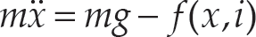
where g denotes the acceleration due to the gravity, and f(x,i) is the magnetic control force, calculated as

f (x, i) = k {(\frac{i}{x})}^{2}

(2)

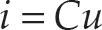
where k is a constant related to the mutual inductance of the ball and coupling coefficients.

The current, i, is linearly related to input voltage u as follows:

i = C u

(3)

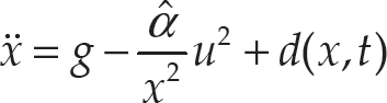
Substituting (2) and (3) into (1) and defining the parameter α = (k ^* C²) / m, we obtain

\ddot{x} = g - \frac{α}{x^{2}} u^{2}

(4)

The parameter α is not precisely known, but it can be obtained by the estimated methods. In addition, Eqs. (2) and (3) can also be obtained by reasonable assumptions. Thus, system (4) can be rewritten in general form as

\ddot{x} = g - \frac{\hat{α}}{x^{2}} u^{2} + d (x, t)

(5)

where $\hat{α}$ is the estimation of α, and d(x,t) is a function of total uncertainty and external disturbance.

Assumption 1: We suppose that the uncertain term is bounded and is given by

| d (x, t) | \leq D

(6)

where D is a positive constant.

The control objective of this article is to design a controller for system (1) such that the output y = x precisely tracks the reference trajectory, x_d(t).

Assumption 2: It is also assumed that x_d(t) ∊ R is a twice continuously differentiable function in terms of t.

3. Design of the AFTC and F-AFTC Controllers for Magnetic Levitation Systems

3.1 Design of Sliding-Mode Surface

We define the tracking error as e(t) = x(t) − x_d(t). Thus, a novel function-augmented sliding hyper-plane, s(t), is defined as follows:

s (t) = ε (t) + \frac{1}{β} \dot{ε} {(t)}^{p / q}

(7)

where ∊(t) = e(t) − v(t), β is a positive constant, and p and q are positive odd integers that satisfy the following condition: 1 < p / q < 2. In addition, ν(t) satisfies the following assumption:

Assumption 3: Considering the augmenting function $ν (t) : R_{+} \to R,$ $ν (t) \in C^{2} [0, \infty), \dot{ν} (t), \ddot{ν} (t) \in L^{\infty},$ the support of ν(t) is a bounded interval [0,T] for T>0, and ν⁽ⁱ⁾(0) = e⁽ⁱ⁾(0)(i = 0,1,2). C²[0,∞) represents the set of all twice continuously differentiable functions defined on [0,∞).

The augmenting function, ν(t), is defined as

ν (t) = {\begin{cases} \sum_{k = 0}^{5} a_{k} t^{k} {\begin{matrix} \begin{matrix}  \end{matrix} \end{matrix}}_{} i f \begin{matrix}  \end{matrix} 0 \leq t \leq T \\ 0 \begin{matrix}  \end{matrix} i f \begin{matrix}  \end{matrix} t > T \end{cases}

(8)

where the coefficients a_k can be found based on Assumption 3. This case involves all six unknown parameters. From Assumption 3, e⁽ⁱ⁾ = ν⁽ⁱ⁾ (i = 0,1,2) gives us three equations:

\begin{array}{l} e (0) = ν (0) \\ \dot{e} (0) = \dot{ν} (0) \\ \ddot{e} (0) = \ddot{ν} (0) \end{array}

(9)

Moreover, Assumption 3 also supposes the continuously differentiable property of the augmenting function, ν(t).

Thus, at instant t = T, three more equations are obtained:

\begin{array}{c} \sum_{k = 0}^{5} a_{k} T^{k} = 0 \\ \sum_{k = 1}^{5} k a_{k} T^{k - 1} = 0 \\ \sum_{k = 2}^{5} k (k - 1) a_{k} T^{k - 2} = 0 \end{array}

(10)

As a result, we can easily find the coefficients a_k as follows:

\begin{array}{l} a_{0} = e (0), a_{1} = \dot{e} (0), a_{2} = \frac{1}{2} \ddot{e} (0), \\ a_{3} = (- \frac{10}{T^{3}} e (0) - \frac{6}{T^{2}} \dot{e} (0) - \frac{3 / 2}{T} \ddot{e} (0)), \\ a_{4} = (\frac{15}{T^{4}} e (0) + \frac{8}{T^{3}} \dot{e} (0) + \frac{3 / 2}{T^{2}} \ddot{e} (0)), \\ a_{5} = (- \frac{6}{T^{5}} e (0) - \frac{3}{T^{4}} \dot{e} (0) - \frac{1 / 2}{T^{3}} \ddot{e} (0)) . \end{array}

(11)

Remark 1: Assumption 3 and the definition in (7) imply that s = 0 at the initial instant.

Remark 2: From Assumption 3 and ∊(t) = e(t) − v(t), it is obvious that $ε (0) = \dot{ε} (0) = 0$ .

3.2 Design of Arbitrary Finite-Time Controller (AFTC)

In order to achieve the control objective for a nonlinear system (5), an arbitrary finite-time control method is described in Theorem 1.

Theorem 1: For ML (5), if the control signal is designed as (12), the tracking error, e(t), will converge to zero in finite time T.

u (t) = \sqrt{\frac{x^{2}}{\hat{α}} (u_{e q} + u_{s})}

(12)

where

u_{e q} = g - {\ddot{x}}_{d} (t) - \ddot{ν} (t) + β \frac{q}{p} {\dot{ε}}^{2 - p / q}

(13)

u_{s} = (D + η) sgn (s)

(14)

Here, η is a positive constant, and

sgn (s) = {\begin{cases} 1 \begin{matrix} f o r \begin{matrix} s > 0, \end{matrix} \end{matrix} \\ 0 \begin{matrix} f o r \begin{matrix} s = 0 \end{matrix}, \end{matrix} \\ - 1 {\begin{matrix}  \end{matrix}}_{} f o r \begin{matrix} s < 0. \end{matrix} \end{cases}

(15)

Proof: Consider the following Lyapunov candidate function:

V = \frac{1}{2} s^{2}

(16)

Differentiating V with respect to time and substituting (5) and (7) into it yields

\begin{array}{l} \dot{V} = s \dot{s} = s (\dot{ε} + \frac{1}{β} \frac{p}{q} {\dot{ε}}^{p / q - 1} \ddot{ε}) \\ \begin{matrix}  \end{matrix} = s [\dot{ε} + \frac{1}{β} \frac{p}{q} {\dot{ε}}^{p / q - 1} (\ddot{x} - {\ddot{x}}_{d} - \ddot{ν} (t))] \begin{matrix}  \end{matrix} \\ = s [\dot{ε} + \frac{1}{β} \frac{p}{q} {\dot{ε}}^{p / q - 1} (g - \frac{\hat{α}}{x^{2}} u^{2} + d (x, t) - {\ddot{x}}_{d} - \ddot{ν} (t))] \begin{matrix}  \end{matrix} \end{array}

(17)

Substituting Eqs. (12), (13) and (14) into Eq. (17) leads to

\begin{array}{c} \dot{V} = s [\dot{ε} + \frac{1}{β} \frac{p}{q} {\dot{ε}}^{p / q - 1} (d (x, t) - β \frac{q}{p} {\dot{ε}}^{2 - p / q} - (D + η) sgn (s))] \\ {\begin{matrix}  \end{matrix}}_{} = \frac{1}{β} \frac{p}{q} {\dot{ε}}^{p / q - 1} [d (x, t) s - (D + η) sgn (s) s] \begin{matrix}  \end{matrix} \end{array}

(18)

Because p and q are positive odd integers and 1 < p / q < 2, then ${\dot{ε}}^{p / q - 1} \geq 0$ . In addition, using Assumption 1, Eq. (18) yields

\dot{V} \leq - \frac{1}{β} \frac{p}{q} η {\dot{ε}}^{p / q - 1} | s | \leq 0

(19)

Therefore, $\dot{V}$ is a negative semi-definite function, i.e., V(t) ≤ V(0). Moreover, from the initial condition, s(0) = 0, as in Remark 1, $V (t) = 0, \forall t \geq 0$ , which is equivalent to $s (t) = 0, \forall t \geq 0$ . From Remark 2, $ε (0) = \dot{ε} (0) = 0$ ; thus, it is easily shown that $ε (t) = 0, \forall t \geq 0$ or e(t) ≡ ν(t). Consequently, if the function, ν(t), is defined as (8), i.e., $ν (t) = 0, \forall t \geq T$ , the tracking error, e(t), will reach zero in finite time T, i.e., $e (t) = 0, \forall t \geq T$ .

This completes the proof of Theorem 1.

Remark 3: It has been shown that $ε (t) = 0, \forall t \geq 0$ indicates the constant existence of the sliding mode with no accompanying reaching phase.

Remark 4: The control effort in Eq. (13) does not include any term that causes the singular problem.

In order to eliminate the chattering phenomenon that is caused by the sign function term in (14), a saturation function is often used to replace the sign(.) function in conventional sliding-mode methods. However, this replacement degrades the tracking performance. In order to overcome this drawback, the fuzzy logic technique is applied.

3.3 Design of Fuzzy-Arbitrary Finite-Time Controller (F-AFTC)

Theorem 2: For ML (5), if the control signal is designed as (20), where u_eq is defined as (13), and k_fs > D, then the tracking error, e(t), will converge to zero in finite time T.

u (t) = \sqrt{\frac{x^{2}}{\hat{α}} (u_{e q} + k_{f s} u_{f s})}

(20)

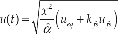
where k_fs is the normalization factor of the output variable, and u_fs is the output of the fuzzy sliding-mode control (FSMC) [9,31]:

u_{f s} = F S M C (s)

(21)

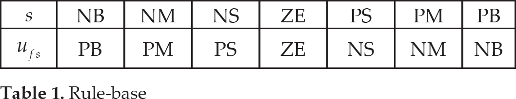
where FSMC(s) presents the functional characteristics of the fuzzy linguistic decision schemes. The input and output variables of FSMC are s (sliding surface) and u_fs. The membership functions of input linguistic variable s and the membership functions of output linguistic variable u_fs are shown in Figure 2. These functions are divided into seven fuzzy functions of negative big (NB), negative medium (NM), negative small (NS), zero (ZE), positive small (PS), positive medium (PM) and positive big (PB). The fuzzy logic system employs the fuzzy rule base in Table 1 [31], the minimum inference engine, the singleton fuzzier, and the centre average defuzzier [32].

Figure 2.

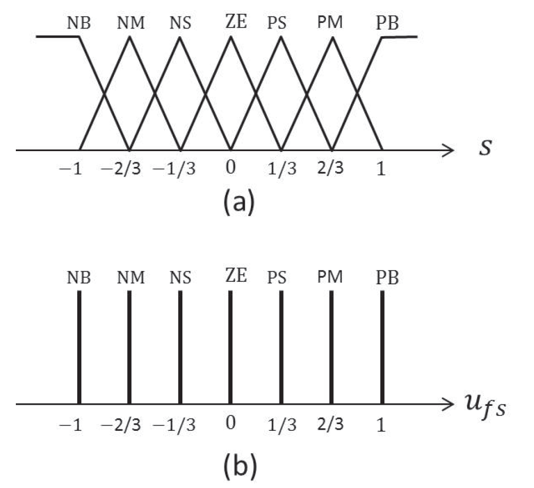
Membership functions of fuzzy sets: (a) input variable and (b) output variable u_fs.

Table 1.

Rule-base

s	NB	NM	NS	ZE	PS	PM	PB
u_fs	PB	PM	PS	ZE	NS	NM	NB

Proof: For Theorem 2, the Lyapunov candidate function is chosen as in (16); we also use the time derivative expressed as Eq. (17). By substituting Eqs. (13) and (20) into (17), with ${\dot{ε}}^{p / q - 1} \geq 0$ , we obtain the following:

\begin{array}{c} \dot{V} = \frac{1}{β} \frac{p}{q} {\dot{ε}}^{p / q - 1} (d (x, t) s - k_{f}_{s} u_{f}_{s}) \\ \leq \frac{1}{β} \frac{p}{q} {\dot{ε}}^{p / q - 1} (D | s | - k_{f s} | s |) \end{array}

(22)

Obviously, if we choose k_fs > D, it can be concluded that $\dot{V} \leq 0$ . Therefore, the analysis is the same as that at the end of subsection 3.2; it is known that the tracking error, e(t), will converge to zero in finite time. The proof of Theorem 2 is known.

4. Numerical Simulation and Experimental Results

In this section, the effectiveness of the proposed AFTC and F-AFTC methods are validated by numerical simulation and experimental study of an ML. For both the numerical simulation and experiment, we consider system (5) with the following nominal parameters [29,30]:

\begin{array}{l} g = {9.81}_{} [(m / s^{2})], C = {1.05}_{} [(A / V)], \\ m = 0.02 [(k g)], K = {2.48315625.10}^{- 5} [(N m^{2} / A^{2})] . \end{array}

(23)

Then, $\hat{α} = {0.00136884}_{} [(N . m^{2}) / (k g . V^{2})]$ . We employ two reference signal types: set-point and sinusoidal trajectory, given by

x_{d}_{1} (t) = 15 (m m)

(24)

x_{d}_{2} (t) = 15 + 3 \sin (0.4 π t) \begin{matrix}  \end{matrix} (m m)

(25)

4.1 Numerical Simulation

In this subsection, simulation results are given to demonstrate the superior performance of the proposed method compared to the TSM method in [25].

Considering system (5), the uncertainty and external disturbance, d(x,t), should be considered. From the experimental results in [30], we assume a real value of α = 0.00134557. Equation (25) implies that x_min = 12(mm), and the control voltage maximum is u_max < 4.5(V). Therefore, a reasonable assumption of the uncertain term is given by

| d (x, t) | \leq \frac{| α - \hat{α} |}{x_{\min}^{2}} u_{\max}^{2} = 3.3 = D

(26)

In this simulation, the initial condition is x₀ = 26(mm). The proposed AFTC method in (12) and the TSM method proposed in [25] are simulated with a set-point reference signal (24).

The TSM controller in [25] is designed as

u = \sqrt{\frac{x^{2}}{\hat{α}} (g - {\ddot{x}}_{d 1} - \ddot{ν} (t) + β \dot{ε} + (D + η') sgn (s))}

(27)

where v(t) is designed as in (8), η′ is a positive scalar, ∊ = e(t) − v(t) = x − x_d1 − v(t), and the sliding surface in this method is $s = \dot{ε} + β ε$ .

For this simulation, to eliminate chatter, the sign(.) function is replaced by a saturation function given by

s a t (\frac{s}{ϕ}) = {\begin{cases} s i g n (s) \begin{matrix}  \end{matrix} i f_{} | s | \geq ϕ \\ \frac{s}{ϕ} \begin{matrix} i f_{} | s | < ϕ \end{matrix} \end{cases}

(28)

where ϕ is a sufficiently small positive constant.

The parameters for both methods are selected as in Table 2. The simulation results are shown in Figure 2. As can be seen in Figure 2, the control performance is good for both methods, and the tracking error approaches zero within T = 0.2(s), which is satisfied according to the chosen convergent time. Thus, our proposed AFTC method is superior to the TSM method in [25] as it has higher-precision tracking, less control effort, and improved behaviour in the transient period. The main reason for these improvements is that our method utilizes a nonlinear hyper-plane as in Eq. (7) instead of a linear hyper-plane as in [25].

Table 2.

Controller parameters for numerical simulation

Control schemes	Parameters
AFTC	T = 0.2, p = 5,q = 3, β = 5; D + η = 4, ϕ = 0.001
TSM [25]	T = 0.2, β = 5, D + η′ = 4, ϕ = 0.001.

Figure 3.

The numerical simulation results of the set point control: (a) output tracking, (b) control input, and (c) sliding surface

4.2 Experimental Results

The ML used in this work and designed by Feedback Instrument [29] is shown in Figure 4. This ML is composed of a mechanical unit (denoted with 1 in Figure 4), an analogue control interface (denoted with 2 in Figure 4), a PCI1711 I/O card (within the computer case in Figure 4), and a feedback SCSI adapter box (denoted with 3 in Figure 4). The control law implemented in the PC uses software tools from MathWorks Inc., such as MATLAB/Simulink, Control Toolbox, Real Time Workshop (RTW), Real Time Windows Target, and Microsoft Visual C++ Professional. The steps necessary to obtain the executable file from the control law model are shown in Figure 5 [29]. The control method is designed in the MATLAB/Simulink environment. Real Time Workshop builds a C++ source program from Simulink. C++ compilers compile and link the code created by RTW in order to produce an executable program. Real Time Windows Target communicates with the executable program and interfaces with the hardware device though the I/O board. Real Time Windows Target manages the two-way signal flow to and from the model and to and from the I/O board.

Figure 4.

Experimental platform

Figure 5.

Tools for control system development

The real values of the experimental platform are as in (23) with a nominal value $\hat{α} = {0.00136884}_{} [(N . m^{2}) / (k g . V^{2})]$ . The experiment describes the implementation of the AFTC method using a saturation function and the implementation of the F-AFTC scheme

The AFTC method (12) is implemented for the reference trajectories, (24) and (25), and the saturation function (28) is employed. The F-AFTC method is designed as in (20). The parameters of the AFTC method and F-AFTC method for the experiment are chosen as in Table 3.

Table 3.

Controller parameters for experiment

Control schemes	Parameters
AFTC	T = 0.2, p = 5, q = 3, β = 5; D + η = 4, ϕ = 0.001
F-AFTC	T = 0.2, p = 5, q = 3, β = 5, k_fs = 10.

The experimental results are depicted in Figure 6 and Figure 7. The results indicate the excellent performance of the proposed AFTC and F-AFTC controllers. It is observed from Figures 6(a) and Figure 7(a) that the convergence time is satisfied, which implies that the actual outputs converge to the reference trajectories within T = 0.2(s). In other words, the system output responses well track the reference trajectories after the finite time, T. However, the tracking performance of the F-AFTC is better than that of the AFTC.

Figure 6.

The set point control for Case E1: (a) output tracking, (b) control input, and (c) sliding surface

Figure 7.

The sinusoidal-trajectory tracking control: (a) output tracking, (b) control input, and (c) sliding surface

Figures 6(c) and 7(c) show the sliding hyper-planes, s(t), which show that the system states are always on in the sliding hyper-plane, i.e., the overall system is in sliding mode all of the time.

5. Conclusions

This article has established the AFTC and F-AFTC methods for tracking control of a real ML. It has been verified that the proposed methods with the novel nonlinear hyper-plane have better performance than the conventional method. The proposed methods not only avoid the reaching-phase problem and the singular problem, but also achieve a highly precise tracking performance. In addition, the controllers cause the tracking errors to converge to zero in finite time, and the relaxation time, T, can be set arbitrarily. This is the first successful implementation of these achievements in a real system. This paper also contributes simpler and more efficient nonlinear control methods that can be employed as good solutions for the stabilization and tracking control of MLs. It should be noted that the proposed method could be easily extended to multi-input multi-output (MIMO) nonlinear systems.

6. Acknowledgements

This work was supported by the Special Research Fund of Electrical Engineering at the University of Ulsan.

References

Kaplan

and Regev

(1976) Dynamic stabilization of tuned-circuit levitators. IEEE Trans. Magn. 12(5): 556–559.

Yamamura

and Yamaguchi

(1990) Electromagnetic levitation system by means of salient-pole type magnets coupled with laminated slotless rails. IEEE Trans. Veh. Technol. 39(1): 83–87.

Dahlen

(1985) Magnetic active suspension and isolation (MS thesis). Dept. Mech. Eng., Massachusetts Inst. Technol., Cambridge, MA.

Park

(1998) Wafer distribution system for a clean room using a novel magnetic suspension technique. IEEE/ASME Trans. Mechatronics. 3(1): 73–78.

Lih-Chang

and Tzyh-Biau

(1997) Feedback linearization and fuzzy control for conical magnetic bearings. IEEE Trans. Contr. Syst. Technol. 5(4): 417–426.

Trumper

Olson

, and Subrahmanyan

(1997) Linearizing control of magnetic suspension systems. IEEE Trans. Contr. Syst. Technol. 5(4): 427–438.

Barie

and Chiasson

(1996) Linear and nonlinear state-space controllers for magnetic levitation. Int. J. Syst. Sci. 27(11): 1153–1163.

Feifei

and Suyama

(1995) Nonlinear feedback control of magnetic levitating system by exact linearization approach. Proceedings of the 4th IEEE Conference on Control Applications. 1995 Sep 28. Albany, NY. pp 267–268.

Kuo

C-L

T-H

, and Guo

(2005) Design of a Novel Fuzzy Sliding-Mode Control for Magnetic Ball Levitation System. Journal of Intelligent and Robotic Systems. 42(3): 295–316.

10.

Cho

Kato

, and Spilman

(1993) Sliding mode and classical controllers in magnetic levitation systems. IEEE Control Syst. Mag. 13(1): 42–48.

11.

Slotine

and Li

(1991) Applied Nonlinear Control. EngleWood Cliffs, NJ: Prentice-Hall.

12.

El-Hajjaji

and Ouladsine

(2001) Modeling and nonlinear control of magnetic levitation systems. IEEE Trans. Ind. Electron. 48(4): 831–838.

13.

Kim

S-W

and Lee

J-J

(1995) Design of a fuzzy controller with fuzzy sliding surface. Fuzzy Sets and Systems. 71(3): 359–367.

14.

Sabanovic

(2011) Variable structure systems with sliding modes in motion control – A Survey. IEEE Trans. Ind. Electron. 7(2): 212–223.

15.

Hung

(1993) Variable structure control: a survey. IEEE Trans. Ind. Electron. 40(1): 2–22.

16.

Al-Multhairi

and Zribi

(2004) Sliding mode control of a magnetic levitation system. Mathematical Problems in Engineering. 2004(2): 93–107.

17.

Shen

J-C

(2002) H∞ Control and Sliding Mode Control of Magnetic Levitation System. Asian Journal of Control. 4(3): 333–340.

18.

Hung

(1993) Variable structure control: a survey. IEEE Trans. Ind. Electron. 40(1): 2–22.

19.

(1998) Terminal sliding mode control design for uncertain dynamic systems. Syst. Control. Lett. 34(5): 281–287.

20.

Park

K-B

and Ju-Jang

(1996) Comments on “A robust MIMO terminal sliding mode control scheme for rigid robotic manipulators”. Automatic Control, IEEE Trans. Automat. Contr. 41(5): 761–762.

21.

Feng

(2009) Hybrid terminal sliding mode observer design method for a permanent-magnet synchronous motor control system. IEEE Trans. Ind. Electron. 56(10): 3424–3431.

22.

Chang

(2008) Real-time implementation of grey fuzzy terminal sliding mode control for PWM DC-AC converters. IET Power Electronics. 1(2): 235–244.

23.

Feng

(2002) Non-singular terminal sliding mode control of rigid manipulators. Automatica. 38(12): 2159–2167.

24.

Yang

and Yang

(2011) Nonsingular fast terminal sliding mode control for nonlinear dynamical systems. Int. J. Robust. Nonlin. 21(16): 1865–1879.

25.

Park

K-B

and Tsuji

(1999) Terminal sliding mode control of second-order nonlinear uncertain systems. Int. J. Robust. Nonlin. 9(11): 769–780.

26.

Perruquetti

and Barbot

(2002) Sliding mode control in engineering. New York: Marcel Dekker.

27.

Furuta

and Pan

(2000) Variable structure control with sliding sector. Automatica. 36(2): 221–228.

28.

Roopaei

(2009) Chattering-free fuzzy sliding mode control in MIMO uncertain systems. Nonlinear. Anal-Theor. 71(10): 4430–4437.

29.

Naumovic

and Veselic

(2008) Magnetic levitation system in control engineering education. Facta Universitatis, Series: Automatic control and robotics. 7(1): 151–160.

30.

Morales

(2011) Nonlinear Control for Magnetic Levitation Systems Based on Fast Online Algebraic Identification of the Input Gain. IEEE Trans. Contr. Syst. Technol. 19(4): 757–771.

31.

Lin

C-M

and Jiun

Fei S

(2000) Adaptive fuzzy sliding mode control for motor-toggle servomechanism. Control Applications, 2000. Proceedings of the 2000 IEEE International Conference on. 2000 Sep 25–27. Anchorage, Alaska, USA. pp. 674–679.

32.

Wang

(1997) A Course in Fuzzy Systems and Control. London, UK: Prentice-Hall. pp. 59–168.

Arbitrary Finite-time Tracking Control for Magnetic Levitation Systems

Abstract

Keywords

1. Introduction

2. System Description and Problem Statement

3.1 Design of Sliding-Mode Surface

6. Acknowledgements

References