Sage Journals: Discover world-class research

Abstract

In the biomedical field, a wireless microrobot in a pipe which can move smoothly in water or other aqueous mediums has been urgently demanded. In this paper, several methods of designing a novel microrobot with symmetrical motion characteristics have been discussed and a new kind of wireless microrobot has been developed. According to the modelling analysis, we considered two kinds of common cases occurring in vertical motion, which required gravity compensation. Based on two groups of simulations and experiments on forward-backward motion, upward-downward motion and inclined plane motion, the results and dynamic error evaluation indicated that the wireless microrobot with symmetrical structure could realize similar kinematic characteristics in the horizontal motion. The gravity compensation played an important role in the design process, and the performance of the vertical motion had been improved by gravity compensation. With this method, we made the wireless microrobot realize symmetrical motion characteristics, and simplified the control strategies. Finally, a control panel for our system was designed, which could control the current motion states more intuitively and far more easily through the buttons. The developed wireless microrobot would be very useful in the industrial application and microsurgery application.

Keywords

Wireless Endoscope Gravity Compensation Symmetrical Motion Characteristics Medical Application

1. Introduction

Endovascular intervention has become more and more popular in recent times. The study of microrobots in a pipe is an important research branch of MEMS (Micro-Electro-Mechanical System). Studies on the locomotion methods of microrobots which move within organic tubes in the human body can be used in practical medical fields, such as diagnosis and treatment of body organs. The traditional endoscopy uses a long, thin and flexible tube which is required for connecting the endoscope with the workstation outside the patient's body [1]. However, the traditional endoscope has two problems, in that they cause pain to the patients and are limited to the view of the small intestine. Therefore, some techniques are required that thoroughly improve the capabilities of the endoscopy field. To minimize the suffering of patients, a capsule endoscope has been developed [2]. With the aid of peristalsis, the capsule moves passively through the GI tract. However, the capsule cannot control its moving direction and moving speed itself, due to the loss of large quantities of data. So the capsule endoscope needs an autonomous moving function.

A number of mechanisms for an actuator have been proposed, which are used for providing locomotion in the pipe, such as piezoelectric elements [3, 4], air cylinders [5], electrorheological fluids [6], shape memory alloys [7, 8], electromagnetic motors [9 –14] and globular magnetic actuators capable of locomotion in a pipe by a combination of mechanical vibration and electromagnetic force [15, 16].

Many studies on the microrobot and microswimmer also had been developed. In 2013, Jian Feng and Sung Kwon Cho proposed a kind of two-dimensionally steering microswimmer propelled by oscillating bubbles [17]. In 2012, Yan-Hom Li and He-Ching Lin proposed a novel steering technology of magnetic micro-swimmers under an oscillating field [18]. In 2011, J. Scogna and J. Olkowski proposed a kind of microswimmer which could be controlled in one dimension for drug delivery and the size was only 7–8 μm [19]. In 2011, Li Zhang and Tristan Petit proposed rotating ferromagnetic nanowires (NWs) which were capable of self-propulsion near a solid boundary using a uniform rotating magnetic field [20].

In our previous study, wireless microrobots controlled by an external magnetic field were safe and reliable, and could be carried deep within the tissues of living organisms in the body fluids. Thus, a new kind of magnetic field model to easily drive the microrobot is required [21–22]. With the different kinds of external magnetic field driven microrobots, many locomotion forms are proposed as shown in Figure 1. For example, the fish-like motion [23], paddle motion [24], propeller-driven motion [25] and spiral motion [26–27]. In many kinds of motions, we identified the kind of spiral motion which not only could obtain the maximum driving force, but also had the highest efficiency in a very small space [28].

Figure 1.

Several kinds of wireless in-pipe microrobots

However, the control algorithm is high level, non-linear and very complex [29], which is mainly due to the asymmetry of kinematic performance. It is also difficult to realize bidirectional motion and upward motion. So in this paper, we focus on developing a kind of wireless microrobot with symmetrical motion characteristics and simplify the control strategies.

2. Rotation Magnetic Field Model

2.1 Design of the Rotation Magnetic Field

The rotation magnetic field model was shown in Figure 2, which contained two pairs of coils. When we inputted the currents with the phase difference of 90° in each coil, the rotation magnetic field was generated.

Figure 2.

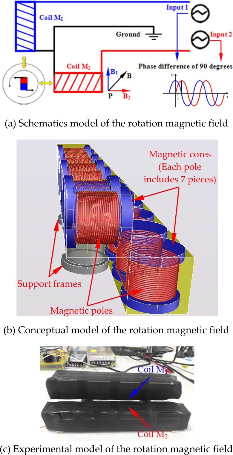
Rotation magnetic field model

We assumed that the currents flowing through the coil M₁ and coil M₂ had the same amplitude, but the phase difference was 90°, which was shown in Figure 2(a). Then the strengths of a magnetic field generated by the coil M₁ and M₂ were given by:

B_{1} = B_{10} \sin ω t

(1)

B_{2} = B_{10} \sin (ω t + 90^{o})

(2)

In order to conveniently analyse the magnetic field, we assumed B₁₀=B₂₀=B₀. The rotation vector directions of B₁ and B₂ were perpendicular to each other, so the absolute value and the direction of the magnetic field after the superposition of the two magnetic field vectors were:

B = \sqrt{B_{1}^{2} + B_{2}^{2}} = \sqrt{{(B_{0} \sin ω t)}^{2} + {(B_{0} \cos ω t)}^{2}} = B_{0}

(3)

\tan θ = B_{1} ∕ B_{2} = \tan ω t

(4)

From the Equation 3 and Equation 4, we could find the value of the synthesis magnetic field strength was a constant, and it was equal to the maximum value B₁ (or B₂). In addition to that, the direction of B changed along with the periodic time changing. So the synthesis of vector B was a rotation vector, and the angular velocity of rotation was ω, which was a rotation magnetic field.

2.2 Parameter of the Rotation Magnetic Field

In our study, we needed to establish a rotation magnetic field to drive the developed microrobot. Based on the magnetic field theory discussed, we had designed a new external superposition magnetic field in horizontal and vertical directions. The experimental model of the rotation magnetic field was shown in Figure 2(c).

We set the two pairs of coil M₁ and coil M₂ at 90° to each other. In order to generate the rotation magnetic field, we made the solenoid by using enamelled wire. In particular, we inserted the magnetic cores to enhance the magnetic flux density. It was a simple design to obtain the rotation magnetic field, and the specification of each coil was shown in Table 1.

Table 1.

Specification of each coil

	Coil M₁	Coil M₂
Turns per coil (times)	150	150
Wire diameter (mm)	0.2	0.2
Length (mm)	210	210
Width (mm)	30	30
Height (mm)	35	35
Resistance (Ω)	10.2	10.4
Magnetic core	Yes	Yes
Size of magnetic core (mm)	Φ30*35	Φ30*35

Following the Biot-Savart Law, the relationship between the magnetic flux density H and current i could be measured by a gauss meter, which was shown in Figure 3, and Equation (5) of the curve could be fitted as well:

Figure 3.

Relationship between the magnetic density and current

H (i) = 2.357 \times 10^{3} \times i

(5)

3. Design of the Microrobot Structure

3.1 The Functional Analysis of the Microrobot

When considering practical application, the microrobot developed should realize the following basic movements:

Moving forward and backward in the horizontal direction

Moving upward and downward in the vertical direction

Stopping and running at any position we need

The microrobot was mainly driven and controlled by an external magnetic field, and the properties of the magnetic field were generated by the current input coil. In order to simplify and optimize the control strategies, the microrobot should have symmetrical motion characteristics.

The symmetrical motion characteristics can be obtained by the most intuitive method, which is the symmetry of the mechanical structure and functions. In addition, as the spiral motion had the highest efficiency in a very small space [21], we should fully consider the symmetrical mechanical structure and the spiral structure.

3.2 The Structure of the Microrobot

The spiral type of microrobot had been designed in our previous study [30], which contained four pieces of permanent magnets and the rotation mechanism was separate with the main body of the microrobot. Based on the analysis aforementioned, we had proposed a new kind of spiral type of microrobot, which only contained one piece of permanent magnet, so it had a more compact structure [31].

Figure 4 s the structure of the prototype of the wireless microrobot. It consists of two main parts. In order to ensure the balance of the microrobot, we adopted a completely symmetrical structure, which also could achieve the same kinematic characteristics. Regardless of the posture and position of the microrobot in the pipe, the centre of mass could always be fixed in the centre of the microrobot (the position of the permanent magnet) as shown in Figure 5.

Figure 4.

The structure of the proposed microrobot

Figure 5.

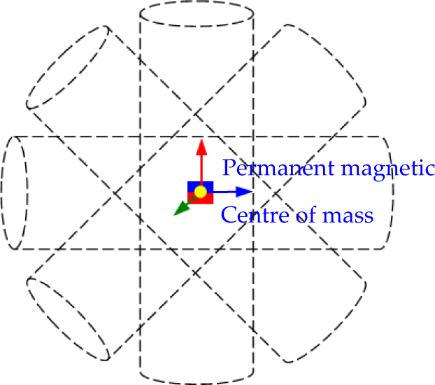
The centre of mass distribution

3.3 The Dynamic Analysis of the Microrobot

With two input currents flowing into the coils, a rotation magnetic field can be generated; the kinematic characteristic of the microrobot are shown in Figure 6. The permanent magnet would rotate following the rotation of the magnetic field. With its spiral structure, the microrobot could thus move forward. By changing the order of the two-phase input currents, we can obtain an opposite direction of rotation of the magnetic field immediately. Then the microrobot would obtain an opposite direction of the driving force and move towards the opposite direction. The moving speed of the microrobot could be controlled by adjusting the frequency of the input currents.

Figure 6.

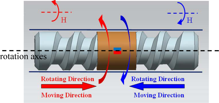
Kinematic characteristics of the proposed microrobot

To propel the wireless microrobot, the propulsive force and torque was provided by rotation of the magnetic field. We could change the magnetic force and torque by following Equation 6 and 7 to overcome fluid resistance in the pipe:

T = μ_{0} V M \times H = V M \times B

(6)

F = μ_{0} V (M \cdot \nabla) \times H = V (M \cdot \nabla) \times B

(7)

where μ₀ is the permeability of vacuum, V represents the volume of the body, M is the average magnetization, ∇ represents a gradient operator, H is the magnetic flux density, B is the magnetic induction intensity.

Due to the symmetrical structure, the propulsive force along the axis could be described by a symmetric propulsion matrix as shown in Equation 8 [32]:

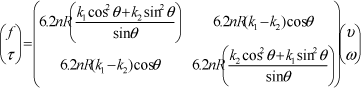
(\begin{matrix} f \\ τ \end{matrix}) = (\begin{matrix} 6.2 n R (\frac{k_{1} \cos^{2} θ + k_{2} \sin^{2} θ}{\sin θ}) & 6.2 n R (k_{1} - k_{2}) \cos θ \\ 6.2 n R (k_{1} - k_{2}) \cos θ & 6.2 n R (\frac{k_{2} \cos^{2} θ + k_{1} \sin^{2} θ}{\sin θ}) \end{matrix}) (\begin{matrix} v \\ ω \end{matrix})

(8)

where, f is the non-fluidic applied force, τ is the non-fluidic applied torque, n is the number of thread units, R and θ are as shown in Figure 8, k₁ and k₂ are the constants, which are the viscous drag coefficients for the wireless capsule microrobot along the axis, υ is forward velocity and ω is angular speed.

Figure 7.

The modelling of the microrobot in the horizontal direction

Figure 8.

The modelling in vertical direction

When the θ was equal to 0 or π, the first and last term in Equation 8 would be zero.

3.4 Modelling and Analysis of the Microrobot

3.4.1 The Modelling in Horizontal Direction

According to the Right-hand Rule, we established the coordinate system for the microrobot movement, which is shown in Figure 7.

In the right-hand coordinate system, V_a was the axial velocity, U_c was the circumferential velocity. In order to simplify the force analysis of the microrobot, we assumed the direction of the screw thread was the x-axis, the thickness direction of the screw thread was the y-axis, the direction which was vertical to the microrobot body was the z-axis, and θ was the spiral angle. U_c and V_a could be composed of u_x (x-component) and ω_z (z-component).

u_{x} = U_{c} \sin θ + V_{a} \cos θ

(9)

ω_{z} = V_{a} \sin θ - U_{c} \cos θ

(10)

Based on Hydromechanical Lubrication Theory and Newton Viscous Law, similar force analysis has been discussed [33], [34]. According to the microrobot we designed in the pipe, the main force would be evaluated as shown in Table 2 in the horizontal direction, which consisted of f_x, f_z, F_axial, F_circum f_l-resist and f_r-fricion.

Table 2.

Explanation of the main force

Force	Explanation
f_x	The total shear stress of the screw thread gap region and the thread region in x-axis.
f_z	The total shear stress of the screw thread gap region and the thread region in z-axis.
F_axial	The axial traction force.
F_circum	The circumferential friction force.
f_l-resist	The resistance from the liquid.
f_r-friction	The rolling friction between the microrobot and pipe.
G	The weight of the microrobot.
F_u	The buoyancy of the microrobot in the liquid.

According to Newton Viscous Law, we could obtain the f_x and f_z as following:

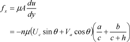
\begin{array}{l} f_{x} = μ A \frac{d u}{d y} \\ = - n μ (U_{c} \sin θ + V_{a} \cos θ) (\frac{a}{c} + \frac{b}{c + h}) \end{array}

(11)

where n is the number of thread unit, μ is the viscosity coefficient of the liquid, A is the contact area, du/dy is the velocity gradient.

f_{z} = - n μ ω_{z} [\frac{3 a b h^{2}}{b c^{3} + a {(c + h)}^{3}} + \frac{a}{c} + \frac{b}{c + h}]

(12)

Then we could compute the axial traction force, circumferential friction force and resistance from liquid as following:

\begin{array}{l} F_{a x i a l} = f_{x} \cos θ + f_{z} \sin θ \\ = \frac{3 n μ a b h^{2} (U_{c} \sin θ \cos θ - V_{a} \cos^{2} θ)}{b c^{3} + a {(c + h)}^{3}} - n μ V_{a} (\frac{a}{c} + \frac{b}{c + h}) \end{array}

(13)

\begin{array}{l} F_{c i r c u m} = f_{z} \cos θ - f_{x} \sin θ \\ = \frac{3 n μ a b h^{2} (U_{c} \cos^{2} θ - V_{a} \sin θ \cos θ)}{b c^{3} + a {(c + h)}^{3}} + n μ U_{c} (\frac{a}{c} + \frac{b}{c + h}) \end{array}

(14)

\begin{array}{l} F_{l - r e s i s t} = 0.5 k ρ V_{a}^{2} S \\ = 0.5 k ρ V_{a}^{2} π R^{2} \end{array}

(15)

F_{r - f r i c t i o n} = η \cdot (G - F_{u})

(16)

G = m_{g} g

(17)

F_{u} = ρ g V_{g} = \frac{ρ}{ρ_{g}} G

(18)

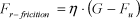
where k is the damping coefficient of the liquid, ρ is the density of the liquid, S is the front of the contact area of the microrobot, η is the coefficient of rolling friction, G is the weight of the microrobot, V_g is the volume of the microrobot, ρ_g is the density of material used to design the microrobot. The m_g can be obtained from an electronic balance easily, then G and F_u can be calculated.

In order to simplify the equations above, we assumed β=a/a+b, γ=h/c, so we could obtain the equations as:

\begin{array}{l} {\bar{F}}_{a x i a l} = F_{a x i a l} \cdot \frac{c}{a + b} \\ = \frac{3 n μ β (1 - β) γ^{3} (U_{c} \sin θ \cos θ - V_{a} \cos^{2} θ)}{(1 - β) + β {(1 + γ)}^{3}} - n μ V_{a} (β + \frac{1 - β}{1 + γ}) \end{array}

(19)

\begin{array}{l} {\bar{F}}_{c i r c u m} = F_{c i r c u m} \cdot \frac{c}{a + b} \\ = \frac{3 n μ β (1 - β) γ^{3} (U_{c} \cos^{2} θ - V_{a} \sin θ \cos θ)}{(1 - β) + β {(1 + γ)}^{3}} + n μ U_{c} (β + \frac{1 - β}{1 + γ}) \end{array}

(20)

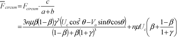
Therefore, the total force of the microrobot in the horizontal direction could be expressed as:

F_{h o r i z o n t a l} = {\bar{F}}_{a x i a l} + {\bar{F}}_{c i r c u m} - F_{l - r e s i s t} - F_{r - f r i c t i o n}

(21)

3.4.2 The Modelling in Vertical Direction

In the vertical motion, we also established the coordinate system for the microrobot's movement as shown in Figure 8. The significant difference was the microrobot was also influenced by its gravity and the buoyancy from the liquid, and the G and F_u should be considered separately.

If we assumed ΔF=F_u-G, the total force of the microrobot in the vertical direction was:

\begin{array}{l} F_{v e r t i c a l} = {\bar{F}}_{a x i a l} + {\bar{F}}_{c i r c u m} + Δ F - F_{l - r e s i s t} - F^{*}_{r - f r i c t i o n} \\ \approx F_{h o r i z o n t a l} + Δ F \end{array}

(22)

F_{r - f r i c t i o n}^{*} = η \cdot {\bar{F}}_{a x i a l}

(23)

As the effect of the F*_r-friction is very small, for the sake of calculation, we assumed F*_r-friction = F_r-friction. Then the F_vertical was only related to F_horizontal and ΔF.

4. Simulation

Due to the symmetrical spiral structure, the microrobot had similar kinematic characteristics in the horizontal direction motion, so we would focus on the study of symmetry motion in the vertical direction.

As a result of the limitation of the external magnetic density, the driving force is also limited. Therefore, there would be two common cases occurring in the vertical direction and needing gravity compensation. One was the F_vertical, a negative value, and the other was F_horizontal, a positive value which was very small. We designed two groups of experiments to illustrate the two cases, and evaluated the motion effects with different design parameters. Firstly, we simulated the performance in the horizontal direction. Secondly, we focused on the simulation in the vertical direction.

4.1 Simulation on Group I

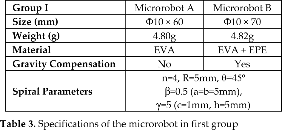
In the first group, we simulated the performance effect of the spiral depth h to F_axial, F_circum, f _l-resist, f _r-friction, F_horizontal and F_vertical. Referring to the structure parameters of the microrobot we developed, as shown in Table 3; it could be assumed β=0.5, μ=1, u=0.005, v=0.05, n=4, k=1, ρ=1, R=0.005, θ=π/4. Considering the size of the microrobot, we fixed the value of γ, ranging from 0 to 10. The simulation results in the horizontal direction are shown in Figure 9 and Figure 10.

Table 3.

Specifications of the microrobot in first group

Group I	Microrobot A	Microrobot B
Size (mm)	Φ10 × 60	Φ10 × 70
Weight (g)	4.80g	4.82g
Material	EVA	EVA + EPE
Gravity Compensation	No	Yes
Spiral Parameters	n=4, R=5mm, θ=45° β=0.5 (a=b=5mm), γ=5 (c=1mm, h=5mm)

Figure 9.

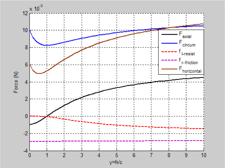
The curves of F_axial, F_circum, f _l-resist, f _r-friction, F_horizontal when γ changes

Figure 10.

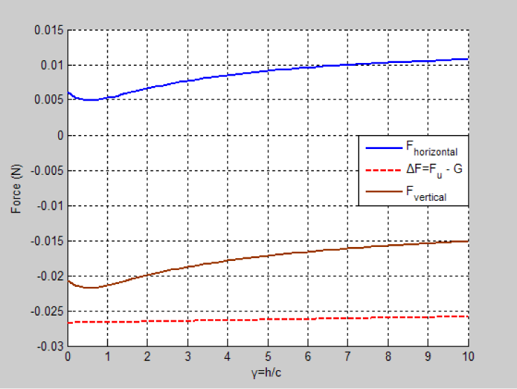
The curves of F_vertical when γ changes

From Figure 9, we can conclude that when h/c>=1 and f_axial>0, the traction force of the capsule was positive, and when h/c=1, f_circum had the minimum value. We could change the value c and h by changing the volume of the microrobot in the different applications. Usually we set a suitable value c, and changed the value of h. The changing of the volume could be approximately neglected because of the small scale of the microrobot.

From Equation 22 and Figure 10, we can find that F_vertical was just related to F_horizontal and ΔF, but the F_vertical was a negative value. So the microrobot could not realize upward motion, and needed gravity compensation.

4.2 Simulation on Group II

In the second group, we simulated the performance effect of the spiral angle θ to F_axial, F_circum, f _l-resist, f _r-friction, F_horizontal and F_vertical. Referring to the structure parameters of the microrobot designed in Table 5, we assumed β=0.5, γ=1, μ=1, u=0.005, v=0.05, n=4, k=1, ρ=1, R=0.003. Considering the size of the microrobot, we fixed the value of θ, ranging from 0° to 90°. The simulation results are demonstrated in Figure 11 and Figure 12.

Table 4.

Specifications of the materials

Part	Material	Density (g/cm³)
Body	EVA	1.1
Permanent magnet	NdFeB	6
Gravity compensation	EPE	0.003

Table 5.

Specifications of the microrobots in the second group

Group II	Microrobot C	Microrobot D
Size (mm)	Φ6 × 50	Φ6 × 60
Weight (g)	1.38g	1.39g
Material	EVA	EVA + EPE
Gravity Compensation	No	Yes
Spiral Parameters	n=4, R=3mm, θ=45° β=0.5 (a=b=5mm), γ=1 (c=3mm, h=3mm)

Figure 11.

The curves of F_axial, F_circum, f _l-resist, f _r-friction, F_horizontal when θ changes

Figure 12.

The curves of F_vertical when θ changes

The simulation results provided the tendency of force applied on the microrobot, which indicated that when θ was from 10° to 80°, the F_vertical was a positive value, but it was a very small value. So the microrobot could achieve upward motion without gravity compensation in theory. When θ was 45°, the microrobot could obtain the maximum total force, so the spiral angle of the microrobot would be designed with 45°.

5. Experimentation

5.1 System Architecture

The experimental system architecture is shown in Figure 13. In the system, the function generator outputted sinusoidal control signals which had a phase difference of 90°. Then by using the amplifying unit, the control signals were able to drive the magnetic field model to generate a rotation of the magnetic field, which controlled the status of the microrobot. During the experiments, we could change the amplitude, frequency and phase of the control signals by adjusting the function generator.

Figure 13.

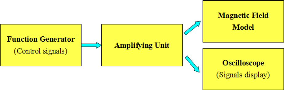
Experimental system architecture

The amplifying unit was an extremely significant part in the system and the circuit is shown in Figure 14. With the aid of the amplifying unit, the weak voltage signal was converted to a strong current signal without any frequency and phase changing. The relationship of conversion could be obtained as following:

Figure 14.

Circuit design of the amplifying unit

I_{o u t} = - \frac{R_{3}}{R_{1}} \cdot \frac{V_{i n}}{R_{r e f}}

(24)

If we choose the R₁=R₂=1Ω, R₃=R₄=10Ω, R_ref=10Ω, the output current would follow with the input signal:

I_{o u t} = - V_{i n}

(25)

5.2 Experiments on Group I

5.2.1 Forward and Backward Motion

In the detection process, the microrobot should complete forward-backward and upward-downward motion in the pipe. Based on the theoretical analysis of the proposed microrobot in our previous study [31], we had proved that it can move forward and backward in a pipe.

By using the measurement system shown in Figure 15, the following characteristics of the moving speed were measured. We carried out the experiments by changing the frequency of input currents from 0 Hz to 20 Hz, and the amplitude of input currents were fixed at 0.7 A.

Figure 15.

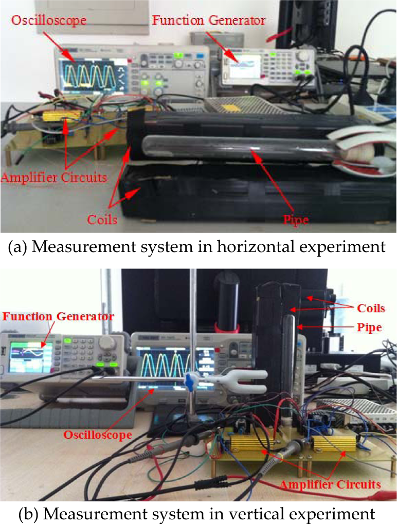
Measurement system

In the first group, the prototype of the developed microrobot (Microrobot A) is shown in Figure 16, and the design parameters are shown in Table 3.

Figure 16.

Prototype of the microrobot

We inserted a piece of axial permanent magnets in the centre of the microrobot body, for which the size was Φ5×2 mm, as shown in Figure 17.

Figure 17.

Prototype of the permanent magnet

Based on the measurement system in Figure 15(a), the microrobot could perform a rotation motion. By changing the frequency and phase of input currents, the moving speed and direction could be adjusted. The experimental results of average moving speed of the microrobot that can be obtained are shown in Figure 18. We had also obtained the maximum moving speed, 22.7 mm/s around 12Hz.

Figure 18.

Moving speed of forward-backward motion

5.2.2 Upward and Downward Motion

According to our preceding analysis and the simulation results shown in Figure 11, the F_vertical was a negative value, so the microrobot could not realize upward motion in theory. We should use a counterweight for the microrobot to make ΔF=0, which could allow the microrobot to suspend in water.

The material of the microrobot body was made of EVA (Ethylene Vinyl Acetate), therefore, we selected another material which had a smaller density as gravity compensation. The specifications of materials are shown in Figure 19 and Table 4.

Figure 19.

The gravity compensation of the microrobot

In addition, the EPE (Expandable Polyethylene) was a kind of soft material, which would be installed at the head and end of the microrobot to buffer the microrobot from impacting with the pipeline. In this way, the safety in the detection process could be improved. The microrobot with gravity compensation (Microrobot B) is shown in Figure 16.

Based on the measurement shown system in Figure 16(b), the microrobot could achieve upward-downward motion in a pipe. The experimental results of average moving speed between the microrobot before and after the gravity compensation are shown in Figure 20.

Figure 20.

Moving speed of upward-downward motion

The experimental results indicated that the microrobot with gravity compensation could realize upward motion easily, and the dynamic characteristics had been clearly improved, which had similar kinematic characteristics in the vertical motion. We had also obtained the maximum moving speed, 6.3 mm/s around 11Hz.

5.2.3 Inclined Plane Motion

In order to evaluate the kinematic characteristics of the microrobot further, we also conducted a set of experiments on the motion with an inclined plane of 45°. The experimental results of average moving speed of the microrobot could be obtained in Figure 21. This indicated that the microrobot with gravity compensation also had similar characteristics in inclined plane motion, and the maximum moving speed was 13.1mm/s around 12 Hz.

Figure 21.

Moving speed of inclined plane at 45°

5.3 Experiments on Group II

5.3.1 Forward and Backward Motion

We reduced the size of the microrobot in order to establish the second case of gravity compensation. The prototype of this microrobot (Microrobot C) is shown in Figure 22, and the design parameters are shown in Table 5.

Figure 22.

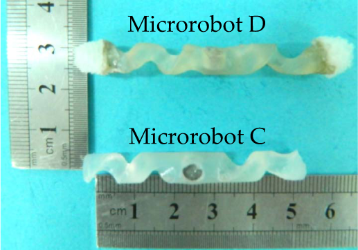
Prototype of the microrobots C and D

Similar to group I, by using the measurement system shown in Figure 15(a), the average moving speed of the microrobot was obtained, as shown in Figure 23. We had also obtained the maximum moving speed, 36.5mm/s around 14Hz.

Figure 23.

Moving speed of forward-backward motion

5.3.2 Upward and Downward Motion

According to the simulation results in Figure 13, we could conclude that when θ was from 10° to 80°, the F_vertical was a positive value, albeit a very small one. The experimental results on upward motion shown in Figure 24 indicate that the microrobot could barely realize the upward motion with a very low speed. In order to simplify the control strategy, we should make the kinematic characteristics as symmetrical as possible, so we also need a counterweight for the microrobot. The microrobot with gravity compensation (Microrobot D) is shown in Figure 22.

Figure 24.

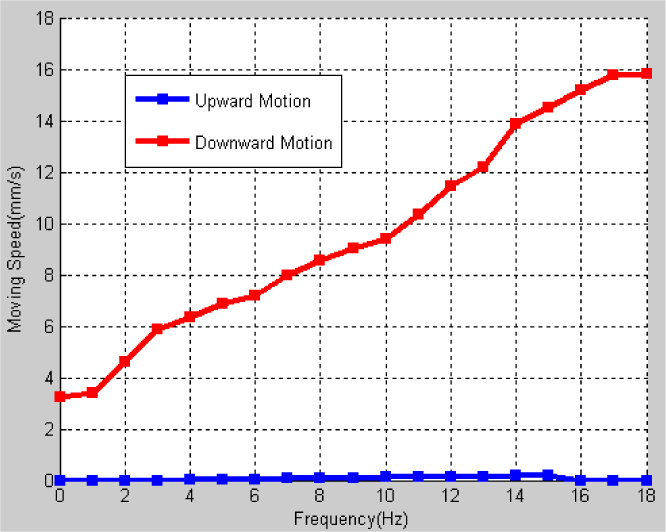
Moving speed of upward-downward motion without gravity compensation

Based on the measurement system shown in Figure 15(b), the experimental results of average moving speed of the microrobot could be obtained as shown in Figure 25, and the maximum moving speed was 4.7mm/s around 16Hz.

Figure 25.

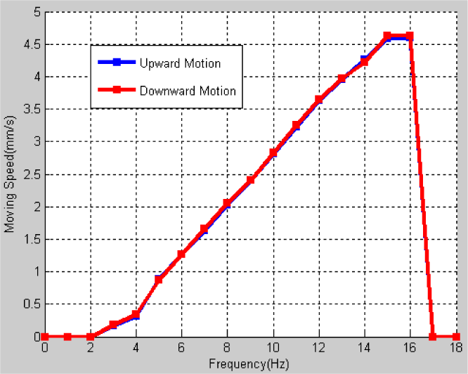
Moving speed of upward-downward motion

5.3.3 Inclined Plane Motion

The experiment of inclined plane motion had also been taken. The experimental results of average moving speed of the microrobot are shown in Figure 26, and the maximum moving speed was 14.8mm/s around 15 Hz. We found that the microrobot with gravity compensation maintained similar kinematic characteristics in the inclined plane motion.

Figure 26.

Moving speed of inclined plane at 45°

5.4 Discussion

We had simulated and experimented, based on the two cases, the effect on the motion performance in the horizontal direction, vertical direction (with or without gravity compensation) and inclined plane motion with gravity compensation. The results are shown in Figure 18, Figures 20–21 and Figures 23 –26.

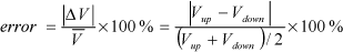
In order to gain a more intuitive evaluated result on the affect of gravity compensation in the vertical motion, we calculated the dynamic error as the following [35]:

e r r o r = \frac{| Δ V |}{\bar{V}} \times 100 % = \frac{| V_{u p} - V_{d o w n} |}{(V_{u p} + V_{d o w n}) ∕ 2} \times 100 %

(26)

The dynamic error analysis and comparison is shown in Figure 27. From Figure 18 and Figure 23, we could conclude that the kind of microrobot we designed realized similar kinematic characteristics in the horizontal direction motion. Furthermore, the ΔF's limited effect on the horizontal motion and the symmetrical structure ensured the centre of mass would always stay at the centre of the microrobot. Viewing the experimental results shown in Figures 20–21 and Figures 25–26, it can be seen that the gravity compensation mechanism would improve the kinematic characteristics in the vertical direction, and the microrobots with symmetrical structure also had similar kinematic characteristics in the vertical motion and inclined plane motion.

Figure 27.

Dynamic error

In addition, we found that the moving speed of the microrobot would decline to zero in the region of high level frequencies in each experimental result. This was because when the applied magnetic field rotated faster than the microrobot's step-out frequency (the frequency requiring the entire available magnetic torque to maintain synchronous rotation), the velocity of the microrobot dramatically declined. So the wireless microrobots could not rotate following the rotation magnetic field at a high level frequency and the velocity would fall to zero [36].

So this new kind of microrobot with symmetrical structure and gravity compensation had the ideal dynamic characteristics for the forward-backward, upward-downward motion and inclined plane motion. The dynamic error of the microrobot with gravity compensation was far less than that of the microrobot without gravity compensation. These advantages would make the control strategies symmetrical and much simpler.

6. Design of control panel for the system

We used a function generator to obtain sine wave signals at the experimental stage, but the device was not portable and compact enough. Due to the symmetrical kinematic characteristics of the microrobot, the control strategies could become symmetrical and much simpler.

Based on the experimental results, the control panel we designed is shown in Figure 28. Through selection of the buttons, we could change the required status of the wireless microrobot. The MCU would output the corresponding signals to the amplifying unit, and then display the current status. The control panel could realize stopping, running and changing the direction of motion, which could be adjusted through the button control. In addition, in the running status, we could choose low-speed motion, mid-speed motion and high-speed motion according to the actual operation needs. The moving speed could be referenced by the experimental results.

Figure 28.

Control panel (Button control: 1. Start/Stop, 2. Motion direction control, 3. Low-speed motion, 4. Mid-speed motion, 5. High-speed motion)

With this control panel, our system would be portable and compact, and we could select the microrobot motion states more intuitively and easily by using the buttons.

7. Conclusion and future work

In this paper, a method to design a microrobot with symmetrical motion characteristics have been discussed and designed. Through modelling analysis, we have considered two kinds of common cases occurring in the vertical motion, which would need gravity compensation. Based on two groups of experiments, the results and dynamic error evaluation have been obtained. This indicated that the wireless microrobot with symmetrical structure would realize similar kinematic characteristics in the horizontal motion, and the gravity compensation would play an important role in the design process. In addition, the kinematic performance of the motion had been improved by a gravity compensation mechanism, which provided the wireless microrobot with symmetrical motion characteristics and simplified the control strategies. At last, a control panel for our system was designed, which would make the current motion states more intuitive and much easier to operate.

The results of two group experiments have been summarized in Table 6. The results indicated that the symmetrical kinematic characteristics of the wireless microrobot in a pipe can be designed following the method we proposed. In addition, we could obtain the ideal dynamic characteristics by the gravity compensation mechanism, especially in the vertical direction motion. These advantages made the control strategies symmetrical and much simpler.

Table 6.

Experimental results

	Group I	Group II
Size	Φ12mm×70mm	Φ6mm×60mm
Weight	4.82g	1.39g
V_{max_horizonal} Frequency	22.7mm/s 12 Hz	36.5mm/s 14 Hz
V_{max_vertical} Frequency	6.3mm/s 13Hz	4.7mm/s 16Hz
V_{max_inclined plane} Frequency	13.1mm/s 12 Hz.	14.8mm/s 15 Hz
Input currents	0.7A	0.7A

In the future, we will focus on establishing a more DOFs experimental system in order to realize the potential for greater microrobot DOFs motion in the pipe, and make it apply to more practical related fields.

Footnotes

8. Acknowledgments

This research is supported by the Key Research Program of the Natural Science Foundation of Tianjin (13JCZDJC26200) and the General Research Program of the Natural Science Foundation of Tianjin (13JCYBJC38600) and The Project-sponsored by SRF for ROCS, SEM.

References

Swain

(2008) The future of wireless capsule endoscopy, World Journal of Gastroenterology. J. 14(26): 4142.

Iddan

Meron

Glukhovsky

and Swain

(2000) Wireless capsule endoscopy, Nature. J. 4: 717–719.

Saito

Sato

Kudo

and Sato

(2000) Fundamental study of mover travel inside a small diameter pipe, Mechanical Engineers. J. 66(641): 346–353.

Fujita

Shiraogawa

Yamamoto

and Kato

(2004) Study of mobile mechanism with elastic fibers by using vibration, Nippon Kikai Gakkai Ronbunshu C Hen. J. 70 (698): 22–26.

Ohno

Hamano

and Kato

(2006) Modeling and fabrication of a mobile inspection microrobot driven by a pneumatic bellows actuator for long pipes, Robotics and Mechatoronics. J. 18(1): 11–17.

Kondo

and Yokota

(1998) Fluid power systems involving the use of an electro-rheological fluid, Society of Mechanical Engineers. J. 64(617): 300–306.

Kwon

Park

Kim

and Park

(2005) Biomaterial property measurement system for locomotive mechanism in gastro-intestinal tract, Proceedings of the 2005 IEEE International Conference on Robotics and Automation, pp. 1315–1320.

Reynaerts

Peilw

and Brussel

(1996) Design of a shape memory actuated gastrointestinal intervention system., Eurosensors X J. pp. 1181–1184.

Zhang

Xie

Wang

(2012) Design, analysis and experiments of a spatial universal rotating magnetic field system for capsule robot, Proceedings of 2012 IEEE International Conference on Mechatronics and Automation, pp. 998–1003.

10.

Miyagawa

and Iwatsk

(2008) Moving characteristics in bent pipes of in-pipe mobile robot with wheel drive mechanism using planetary gear drive, Japan Society for Precision Engineering. J. 74(12): 1346–1350.

11.

Bocko

Kelemen

Kelemenova

and Jezny

(2009) Wheeled locomotion inside pipe, Bulletin of applied mechanics. J. 5(18): 34–36.

12.

Choi

and Roh

(2007) In-pipe robot with active steering capability for moving inside of pipelines, Bioinspiration and Robotics. J. 23: 375–400.

13.

Suzumori

Wakimoto

and Tanaka

(2003) In pipe inspection micro robot adaptable to changes in pipe diameter, Robotics and Mechatronics. J. 15(6): 609–615.

14.

Brunete

Torres

Hernando

and Gambao

(2006) A 2 DoF servomotor based module for pipe inspection modular micro-robots, Proceedings of the 2006 IEEE/RSJ International Conference on Intelligent Robots and Systems, pp. 1329–1334.

15.

Yaguchi

and Sato

(2010) Globular magnetic actuator capable of free movement in a complex pipe, Magnetics. J. 46(6): 1350–1355.

16.

Yaguchi

Sato

and Shikoda

(2011) Magnetic actuator group of globular type capable of free movement in a complex pipe, Magnetics. J. 47(10): 4159–4162.

17.

Feng

and Cho

S. K.

(2014) Two-dimensionally steering microswimmer propelled by oscillating bubbles. Proceeding of the 2014 IEEE 27th International Conference on Micro Electro Mechanical Systems, pp. 188–191.

18.

Scogna

Olkowski

Fatema

Parameswaran

and Dhillon

(2011) Biologically Inspired Robotic Microswimmers. Proceeding of the 2011 IEEE 37th Annual Northeast Bioengineering Conference, pp. 1–2.

19.

Lin

, and Chen

(2011) Steering of magnetic micro-swimmers, Magnetics. J. 49 (7): 4120–4123.

20.

Zhang

Petit

Peyer

, and Nelson

(2011) Nickel nanowire swimmers for colloidal cargo transport near a solid surface. Proceedings of the 2011 International Conference on Nanotechnology, pp. 307–312.

21.

Sendoh

Ishiyama

and Arai

K. I.

(2002) Direction and individual control of magnetic micromachine, Magnetics. J. 38: 3356–3358.

22.

Tan

Liu

(2011) Experimental investigation of the small intestine's viscoelasticity for the motion of capsule robot, Proceedings of the 2011 IEEE International Conference on Mechatronics and Automation, pp. 249–253.

23.

Guo

Sasaki

and Fukuda

(2003) A new kind of microrobot in pipe using driving fin, Proceedings of the 2003 IEEE/ASME International Conference on Advanced Intelligent Mechatronics, pp. 667–702.

24.

Pan

and Guo

(2009) A Paddling type of microrobot in pipe, Proceedings of the 2009 IEEE International Conference on Robotics and Automation, pp. 2995–3000.

25.

Guo

and Pan

(2007) Mechanism and control of a novel type microrobot for biomedical application, Proceedings of the 2007 IEEE International Conference on Robotics and Automation, pp. 187–192.

26.

Guo

Pan

and Khamesee

M. B.

(2008) Development of a novel type of microrobot for biomedical application, Microsystem Technologies. J. 14(3): 307–314.

27.

Pan

Guo

and Okada

(2011) A novel hybrid wireless microrobot, Mechatronics and Automation. J. 1(1): 60–69.

28.

Okada

Guo

and Xiao

(2012) Control of the wireless microrobot with multi-DOFs locomotion for medical applications, Proceedings of 2012 IEEE International Conference on Mechatronics and Automation, pp. 2405–2410.

29.

Zhang

Y. S.

Wang

and Du

C. Y.

(2013) Control theorem of a universal uniform-rotating magnetic vector for capsule robot in curved environment, Science China Technological Sciences. J. 56(2): 359–368.

30.

Pan

and Guo

(2008) Development of a spiral type of wireless microrobot, Proceedings of the 2008 IEEE/ASME International Conference on Advanced Intelligent Mechatronics, pp. 813–818.

31.

Guo

and Wei

(2013) Development of a New Kind of Magnetic Field Model for Wireless Microrobots, Proceedings of the International Conference on Complex Medical Engineering, pp. 580–585.

32.

Guo

and Yamauchi

(2013) Characteristic evaluation of a wireless capsule microrobotic system. Proceedings of the 2013 IEEE International Conference on Mechatronics and Automation, pp. 831–836.

33.

Zhang

and Zhang

(2006) Spiral drive characteristics of a micro robot inside human body, Robot. J. 28: 560–570.

34.

Guo

Wei

and Guo

(2013) Performance evaluation of the wireless microrobot in pipe with symmetrical spiral structure. Proceeding of 2013 IEEE International Conference on Robotics and Biomimetics, pp. 1252–1257.

35.

Fang

(2006) Uncertainty analysis on error, relative error and the error of the reference, Industrial Measurement. J. 16(3): 40–43.

36.

Mahoney

A. W.

Nelson

N. D.

Peyer

K. E.

(2014) Behavior of rotating magnetic microrobots above the step-out frequency with application to control of multi-microrobot systems, Applied Physics Letters. J. 104(14): 144101.

Development of Wireless Endoscope with Symmetrical Motion Characteristics

Abstract

Keywords

1. Introduction

2. Rotation Magnetic Field Model

2.1 Design of the Rotation Magnetic Field

2.2 Parameter of the Rotation Magnetic Field

3. Design of the Microrobot Structure

3.1 The Functional Analysis of the Microrobot

3.2 The Structure of the Microrobot

3.3 The Dynamic Analysis of the Microrobot

3.4 Modelling and Analysis of the Microrobot

3.4.1 The Modelling in Horizontal Direction

3.4.2 The Modelling in Vertical Direction

4. Simulation

4.1 Simulation on Group I

4.2 Simulation on Group II

5. Experimentation

5.1 System Architecture

5.2 Experiments on Group I

5.2.1 Forward and Backward Motion

5.2.2 Upward and Downward Motion

5.2.3 Inclined Plane Motion

5.3 Experiments on Group II

5.3.1 Forward and Backward Motion

5.3.2 Upward and Downward Motion

5.3.3 Inclined Plane Motion

5.4 Discussion

6. Design of control panel for the system

7. Conclusion and future work

Footnotes

8. Acknowledgments

References