
Abstract
Genetic algorithm (GAs) have attracted considerable interest for their usefulness in solving complex robot path planning problems. Specifically, researchers have combined conventional GAs with problem-specific operators and initialization techniques to find the shortest paths in a variety of robotic environments. Unfortunately, these approaches have exhibited inherently unstable performance, and they have tended to make other aspects of the problem-solving process (e.g., adjusting parameter sensitivities and creating high-quality initial populations) unmanageable. As an alternative to conventional GAs, we propose a new population-based incremental learning (PBIL) algorithm for robot path planning, a probabilistic model of nodes, and an edge bank for generating promising paths. Experimental results demonstrate the computational superiority of the proposed method over conventional GA approaches.
1. Introduction
GAs [1], which mimic the genetic evolutionary processes found in nature, comprise one of the most commonly used modern stochastic optimization algorithms. It has been applied to problems in bioinformatics [2], financial mathematics [3], and power electronics design [4]. Over the last decade, GAs have gained popularity within the intelligent robotics community as a method for solving the robot path planning problem, which involves finding the shortest path from a starting point to a destination point while negotiating intervening obstacles. The conventional GA procedure can be summarized as follows: (1) Generate an initial population that contains random representatives of candidate solutions. (2) Crossover and mutate the representatives within the population to create new representatives. (3) Alter the population using the newly created representatives. (4) Repeat steps (2) and (3) until termination conditions are satisfied. Upon termination, the representative with the highest level of fitness is considered the solution.
To date, a number of studies have proposed methods for solving robot path planning problems using conventional GAs [5–10]. Unfortunately, the performance of these methods depends greatly the upon population size and the number of iterations, as the GA may be unable to find a qualified path within the designated number of iterations or else may end up with a path of relatively low quality. Although researchers have tried to improve conventional GAs by introducing problem-specific operators [11–20] and initialization techniques [15–17, 21–23], the high number of parameters required by these operators has limited any performance improvements, as well as creating new problems for population initialization.
In this paper, we propose a robot path planning algorithm that uses a PBIL technique [24–26]. To the best of our knowledge, our algorithm is the first attempt to apply PBIL in the field of robot path planning. The strength of PBIL lies in its well-known capability in finding near-optimal solutions in the region of convergence within a manageable period [24]. Our approach combines the genetic evolutionary process with a probabilistic distribution model to produce an optimized path. To solve the path planning problem efficiently, we also propose a probabilistic model of nodes that maintains information on dominant nodes in the most promising paths during the iterative evolutionary processes, and describe the use of an edge bank for storing the most qualified edges. Our approach significantly reduces the complexity of genetic algorithmic design, thus minimizing the parameters for optimization and achieving significant performance improvements. A series of robot path planning experiments demonstrate the advantages of the proposed method over conventional GAs.
The remainder of this paper is organized as follows. Section 2 discusses previous milestones in the incorporation of GAs into the field of robot path planning. Section 3 describes the proposed method. Section 4 presents experimental results. Finally, Section 5 provides some concluding remarks.
2. Related works
Previous research into applying GAs to path planning problems can be divided into (1) map and path representation [8–14, 16, 17, 19, 20], (2) the design of genetic and problem-specific operators [11–20], and (3) the creation of an initial feasible path set [15–17, 22].
In their map representation approach, Tu and Yang [8] designed a map using nodes numbered with four-bits, where the first three bits denoted one of eight directions, and the last bit flagged the possibility of moving to adjacent nodes. Naderan-Tahan and Manzuri-Shalmani [16] designed a path using a connected Cartesian floating point representation. Shi and Cui [9] modelled a path as a combination of support points derived orthogonally from equidistant segments of the path for obstacle avoidance. Shamsinejad et al. [10] designed a map as a sequence of nodes with a specified distance and direction to the next node. More recent research has represented paths using a sequential list of decimal-numbered nodes [11–14, 17, 19, 20], and presented a map in the form of a grid, indexed by decimals, such that the combination of each cell and its number on the grid can represent a path between the starting and destination nodes. This representation has several benefits, including path-intuitiveness and ease of implementation. Recognizing this, we have also chosen to represent maps and paths as sequential lists of decimal-numbered nodes.
Many researchers have created knowledge-based GAs (KGAs) by adding new operators for obstacle avoidance. Gemeinder and Gerke [11] modified the mutation and crossover operators, and added a tighten operator for optimizing paths with respect to their length. Hu and Yang [12, 13] proposed the use of domain knowledge in designing genetic operators for path planning and developed three problem-specific operators (repair, delete and improve) as examples. Li et al. [15] proposed a repair operator that introduces two new edges to an infeasible edge, allowing it to avoid obstacles. Yun et al. [17] used a delete operator that removes any nodes connected by two edges if the length of the new edge is shorter than the sum of the lengths of the original two edges.
Naderan-Tahan and Manzuri-Shalmani [16] replaced a mutation operator with operators that change (i.e., replace a randomly selected node with an adjacent node in a pre-defined radius), smooth (i.e., eliminate sharp turns) and short-cut (i.e., remove redundant nodes) operators. Yao and Ma [18] and Tuncer and Yildirim [20] also designed new mutation operators by changing the strategy for selecting random nodes for mutation. Tsai et al. [19] developed add and delete operators based on the B-spline smoothing technique to repair paths by inserting a node between any two nodes and deleting a randomly selected node.
Despite these innovations, the KGA continues to be limited by its algorithmic complexity and excessive parameterization. Because suitable values for parameters are generally unknown in practical contexts, additional processing is required, thus creating performance instabilities.
GAs can also be used to modify the initial path set creation process via feasible population-based GAs (FGAs) [15–17, 22]. Classical GAs create an initial path set based on randomly selected nodes on the map, whereas FGAs use additional techniques to reconfigure the infeasible paths in the randomly selected initial path set into feasible paths, allowing faster convergence toward a solution set.
Li et al. [15] introduced an obstacle avoidance algorithm specifically designed for creating the initial path set. This algorithm creates a path by connecting the start and destination points, and then adds several new points to avoid obstacles. Yun et al. [17] also developed an obstacle avoidance algorithm (OAA) as well as a distinguish algorithm (DA) to create the initial paths. If an edge along a path intersects any obstacle, the OAA redirects the edge in question towards any free space in a vertical or horizontal direction, while the DA helps to distinguish the overall feasibility of the path.
Naderan-Tahan and Manzuri-Shalmani [16] introduced a feasible path set creation process that uses a clearance-based probabilistic roadmap method (CBPRM) to obtain collision-free paths under two constraints: (1) the next node should be selected such that it is closer to the destination than the current node, and (2) the line segment that links the current node and the next node must not contain obstacles. Zhao et al. [22] proposed a feasible path set creation method based on three priority groups of adjacent nodes aligned in eight directions. The method creates feasible paths by observing the selection frequency of adjacent nodes.
The limitation of FGA techniques lie in their practical computational costs when revising multiple infeasible paths [15, 17, 22], and in their lack of generality when applied to various map configurations [15–17].
The PBIL algorithm was first introduced by Baluja, who clarified its advantages over conventional evolutionary algorithms [24–26]. PBIL is now known to find near-optimal solutions in the region of convergence within a reasonable amount of time, obviating further operators, parameters and complexity:
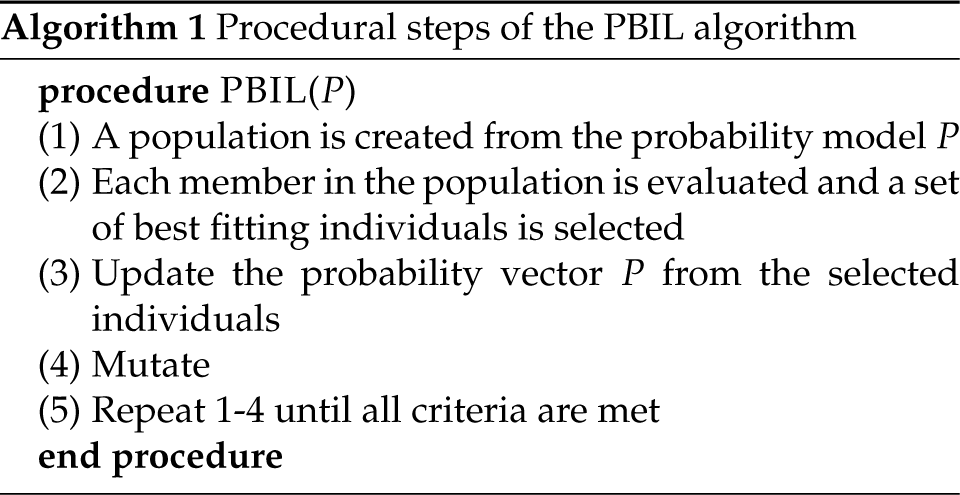
The basic steps of the PBIL algorithm are shown in Algorithm 1 [24]. Note that the work flow of PBIL is similar to that of GAs, except that the PBIL algorithm constructs a probability model for the best past individuals and uses this model to generate the next population. PBIL creates a set of individuals according to the probability model P. Each individual is assessed using an evaluation function and individuals with a high fitness value are selected. Based on the modification rule, the algorithm updates the probability model P based on the posterior probability model implied from the selected individuals. The PBIL algorithm also uses mutation to preserve the diversity of representatives. This procedure is iteratively applied until termination conditions are satisfied.
Herein, we propose a special use of the PBIL algorithm for robot path planning (ROBIL). To improve the performance of ROBIL, we also propose a probabilistic node model and an edge bank for storing information on dominant nodes and edges along feasible paths. During the iterative evolutionary process, the node model stores the probabilistic values of nodes found most frequently along promising paths, and the edge bank stores edge information found along good paths.
3. Proposed method
3.1. Path representation and evaluation function
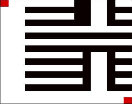
In this section, we represent a map and path as shown in Figure 1. We divide the map into n by n grids, and denote a cell on a grid as node i = 1,2,…,n2, such that a path is composed of the starting node, the destination node, and multiple passage nodes that are candidates to belong to the final path, which may vary according to the path they lie along. Path k can then be represented as a variable-length vector of sequential nodes, Sk = < s1, s2,…,sL+1 >, for which s1 and sL+1 are always the starting and destination nodes, respectively, and s2,…,sL are passage nodes. For example, in Figure 1, white nodes represent obstacle-free spaces, black nodes represent obstacles, red nodes represent the starting and destination nodes, and yellow nodes represent the passage nodes. Hence, a path generated randomly, which starts from node 1 and ends with node 100, can be represented as a vector, S1 =< 1, 5, 47, 44, 74, 96, 100 >. The number of paths, i.e., the size of the population, is fixed at m, |S| = m. Path k has a set of edges, Lk, and any edge, eij ∈ Lk, represents an edge linking two nodes, si and sj, on a path Sk.
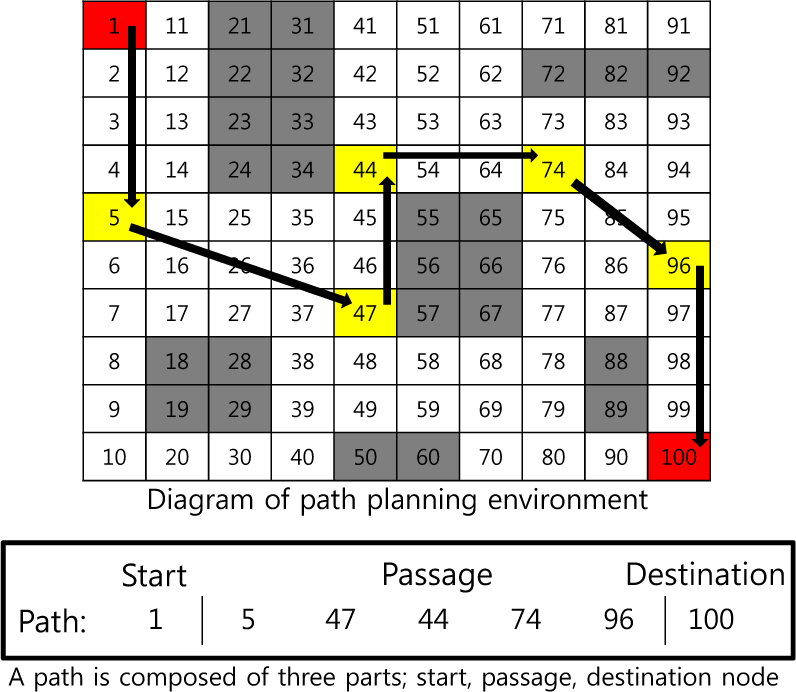
Map encoded from an environment and an example path
The evaluation function is designed to assess the fitness or quality of a given path, Sk, using a common evaluation function [8]. The length of a path is obtained by calculating the sum of the lengths of the edges involved. If any edge contained in a path intersects any obstacles, a penalty is added to the fitness value. This can be written as:

In equation (1), E(Sk) denotes an evaluation function that calculates the fitness value of a given path, Sk, and dis(Sk) denotes the sum of the Euclidean distance of edges along the path, Sk. This can be written as:

In equation (2), the term euc(eij) denotes the Euclidean distance of an edge linking nodes si and sj. The term hin(Sk) is defined as:

The parameter Γ denotes the weight of a penalty, and β(eij) denotes the number of obstacle nodes intersected by edge eij. If the edge eij does not intersect any obstacle, then β(eij) will be zero. Since all the algorithms in our paper use the same fitness function for their path evaluation, the weight of the penalty, Γ, can remain constant.
3.2. Design of a probabilistic node model
A flow chart of the proposed PBIL-integrated algorithm is provided in Figure 2. Based on our assumption that nodes frequently occurring on paths with low evaluation scores indicate a higher probability of a feasible path, we construct a node probability model, P, which stores the probabilistic values of nodes frequently found on promising paths. Hence, the probability of each node in a probability model P represents the selection opportunity for that node to be used to create a new promising path.
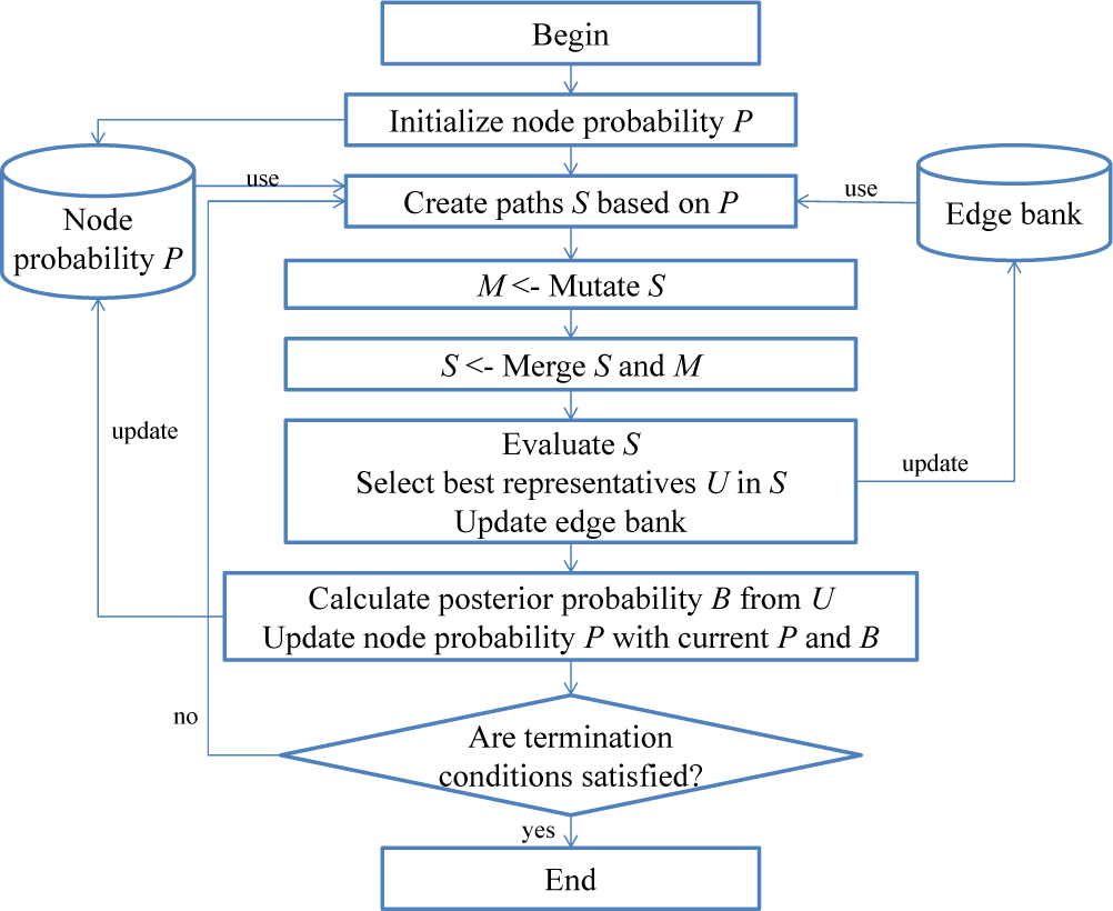
Flowchart of the proposed ROBIL algorithm
Let vector P =< p1, p2, …, pn2 > be the probability model for the path planning problem, where pi denotes the selection probability of a node i. The algorithm initializes the selection probability pi to 0.5 if the node corresponding to pi is in a free space. Thus, nodes within the free space of a map can be randomly selected.
Figures 3 and 4 illustrate the initial and termination states of our probability model. The selection probability of each node is configured to 0.5 when the algorithm initializes the probability model, as shown in Figure 3. The starting, destination and obstacle nodes are represented as S (red node), D (red node), and grey nodes, respectively. Note that the selection probability of S, D and the obstacle nodes are set to zero. After a number of iterations, the selection probabilities corresponding to frequently selected nodes in newly created paths with a higher fitness will have increased. Figure 4 shows the probability model when the iteration has terminated; yellow nodes represent the nodes contained in the obtained path. The results show that the probability of the infrequently selected nodes converges to zero and that the probability of the frequently selected nodes increases. Therefore, the selection probability of the nodes that lie along S to D can be larger than zero, but they still may not be included in the obtained path because of their fitness value. The probabilistic model of the nodes does not provide specific sequence (path) information of the selected nodes; it maintains a set of dominant nodes in the most promising paths. Therefore, a mechanism for creating and improving a path from P by connecting selected nodes is required (in Section 3.3).

Initial probability model
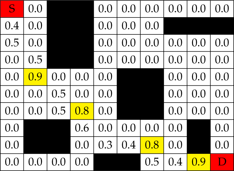
An example of a probability model after termination
Let us explain the design of a probabilistic model in detail. First, our algorithm creates the path set S using the probability model P until the number of paths is satisfied. The procedural steps for creating Sk ∈ S are as follows. Because there is no prior knowledge regarding the number of nodes in Sk, the algorithm randomly chooses the number of nodes to be appended. Afterwards, the algorithm selects a node i from the given map randomly. Next, a random number υ ∈ [0, 1) is produced to determine whether the node i will be appended to Sk. Two probability values, pi and υ, are compared to append a randomly selected node i to Sk. If pi is larger than υ, then the node i is appended as a node element to path Sk; the node i has a high probability of being a passage node in the best path. Moreover, it can allow a random walk on a solution path to some extent, which imposes a flexibility to the path improvement. Conversely, if pi is smaller than υ, then the node i is discarded. These procedures for creating Sk are repeated until all possible nodes of the given map are tested, with the edge bank guiding path-improvement.
The mutation operator is then used on S to obtain a genetically mutated path set M. To find additional useful edges and increase the diversity of the path set, we employed the mutation operator that was used in [12]. This mutation operator chooses a node of Sk ∈ S randomly and replaces it with a free node that is not included in the path. Because the mutation operator cannot guarantee that a newly created path is always superior to the original path, the algorithm merges S and M to prevent the loss of superior paths, i.e., S ← S ∪ M.
Next, the algorithm evaluates the fitness of the paths in S. Once the paths with the best fit, U, are selected based upon their fitness value with a roulette-wheel selection method, the posterior probability model B for the selected paths U is calculated and used to update the probability model P. The equation for updating the probability model is given by:

The term pinew is updated using the selection probability piold of node i in the previous generation and a posterior selection probability bi of node i in the current generation. The posterior probability of nodes B indicates the selection ratio of the nodes in the fittest paths of the current generation. It uses a vector-based representation, B = < b1, b2,…, bn2 >, where bi denotes the selection probability of node i.
The learning rate, LR, is used to control the learning balance between the current probability distribution of nodes P and the posterior probability distribution B. For example, if LR is set to zero, then P cannot converge further because the posterior probability B does not influence P. As a result, the algorithm chooses a node for creating S randomly because the selection probabilities pi ∈ P are set to 0.5 in the initialization step and do not change during the evolutionary processes. Conversely, if LR is set to one, then the selection probabilities of all the nodes that are not selected in the first iteration will be zero because the algorithm is only influenced by the posterior probability model B. Therefore, the algorithm will have difficulty considering the set of nodes that are necessary to create the fittest paths during its remaining iterations.
To construct B, a path set U from path set S is selected according to the roulette-wheel selection method based on score metrics, and the size of the path set U is then fixed at m, |U| = m. In the selected path set, U, the occurrence frequency and average of each node, i, bi, are calculated as shown in Equation (5). Here, occur(Uj, i) returns 1 if node i occurs in path Uj; otherwise, 0 is returned. Thus, each bi (0 ≤ bi ≤ 1) in B indicates how often a node occurs in the selected paths, which paths were evaluated as promising, and how significantly a node can contribute to the construction of an optimal path:

3.3. Creating a path with an edge bank
Although the probability model efficiently reduces the number of nodes that the algorithm considers in creating a path, it does not provide any information on the proper sequencing of selected nodes, so as to avoid intervening obstacles. We therefore introduce an edge bank for storing a set of safety edges from which feasible paths may be more efficiently created.
Figure 5 shows an example of an edge bank construction and update process performed during a path evaluation, as illustrated in Figure 2. The example path in Figure 5 is composed of three nodes: 1, 20 and 36. There are two edges, (1, 20) and (20, 36), the first of which is feasible and the second of which is infeasible. The algorithm stores edge (1, 20) in the edge bank, and discards edge (20, 36). It can then use the stored “safety edges” to create new paths with a higher chance of feasibility.

Example of the construction and updating of the edge bank
Figure 6 illustrates the creation of a new path. The generation of new paths S relies on both the edge bank and the probability model, as shown in Figure 2. The algorithm first configures a new path, Sk, using the probability model P to ensure the selection of promising nodes. The algorithm then amends path Sk to path Sk′ to use the safety edges stored in the edge bank.

Example of new path generation using the edge bank
Because the path starts with node 1, the algorithm begins by finding the safety edges that contain query node 1 in the edge bank (Step 1). We can see that there are two safety edges that start with node 1, (1, 16) and (1, 27). Because node 16 is already used in path Sk, the algorithm selects the safety edge (1, 16) to form a new modified path, Sk′. Next, nodes 1 and 16 are deleted from path Sk, and node 16 is set as a new query node (Step 2). The algorithm then searches for new safety edges starting with node 16. Finding no such safety edges in the bank, the first node among the remaining nodes in path Sk is attached to path Sk′. Node 48 is then set as the new query node (Step 3). The algorithm finds a safety edge (48, 42), but node 42 is not a member of path Sk. Hence, the algorithm attaches node 80 at the tail of path Sk′. Because there is a safety edge connected to the destination node (80, 100), the algorithm ends the creation process, and replaces path Sk with path Sk′ (Step 4). As a result, path Sk, generated based on the probability model P, is amended to create a new path Sk′ in which some of the selected nodes are linked with safety edges and are therefore more likely to form a feasible path.
The detailed process of path creation using an edge bank is shown in Figure 7. The algorithm begins by creating a path based on the probability model and copies the starting node to the head of a new empty path. This first node becomes the initial query node for finding safety edges that start with this node and end with any node on the original path. If any safety edge is found, the algorithm attaches the latter node of the safety edge to the new path. If no safety edges are found for the initial query node, the head of the remaining node from the original path is attached to the new path. Nodes included in the new path are then deleted from the original path. This process is repeated until all the nodes in the created path are considered or else the path is connected to the destination node.

Flowchart of the path creation process
The edge bank used to store safety edges in the path creation process may store n4 possible edges for a given map, in the worst case, if there is no obstacle node. Therefore, the space complexity of ROBIL is O(n4). This is the same as the space complexity of Dijkstra's algorithm, O((the number of nodes)2)=O((n2)2).
4. Experimental results
To verify the effectiveness of the proposed ROBIL method, we compare its performance with that of a well-known KGA [12] against six conventional maps (shown in Figure 8) used in previous studies [12, 13]. Each map consists of a 16 × 16 grid. The simulation was performed on a 2.50 GHz Intel Core i7 with 2 GB of memory, running a MATLAB 7.0 environment.

Six maps used in comparison results
To create an initial population with feasible paths, we implemented three well-known FGA approaches by Li [15], Yun [17] and Naderan-Tahan [16], and conducted a series of experiments. Because of their inherent inefficiencies and lack of generality, however, these approaches took over five minutes to create their initial populations, even for our simple conventional maps [15, 17], and failed altogether for certain map configurations [15–17]. In contrast, the GA, KGA and ROBIL do not incur FGA initialization problems because they create the initial population or the model of the node selection probability randomly. We therefore excluded the experimental FGA results from our comparison.
4.1. Parameter selection
A path planning algorithm achieves its goal by finding a feasible path. Hence, each parameter used in the three algorithms was selected based on the success rate, i.e., the ratio of feasible paths found to the number of attempts. The size of the path set was configured to 50, |S| = 50, and the maximum number of iterations allowed was set to 100. Given the stochastic nature of evolutionary algorithms, we conducted each experiment 20 times for each set of parameter values, and measured the performance as the average success rate.
Figure 9 shows a coloured-contour plot of the success rates for Map 5 for different ROBIL parameters. The horizontal and vertical axes represent the mutation and learning rates, respectively. The boundaries of the two parameters are 0.1 through to 0.9, and the corresponding success rate is between 0 and 1. A high success rate is shown in red, and a low success rate is shown in blue. In Figure 9, we can see that the best success rate can be obtained when the mutation rate is below 0.4 and the learning rate is either 0.1–0.2 or 0.4–0.7. Table 1 shows the success rates of ROBIL for Map 5 with different mutation rates, with the learning rate set to 0.2. From Table 1, we can see that ROBIL found a stable solution in all 20 trials on Map 5, when the learning rate was set to 0.2 and the mutation rate was set to 0.2, 0.6, 0.7 and 0.9, respectively. This tendency is observed consistently for the other maps. Thus, we set the mutation and learning rates of ROBIL to 0.2 in our experiments.
The success rates of ROBIL for various mutation rates (M) when the learning rate (L) is set to 0.2


Parameter selection for ROBIL on Map 5
The parameters used in each algorithm influence each other, creating intractable computational costs for obtaining the best values of various parameters. We therefore describe each algorithm's parameters using a greedy approach. Table 2 shows the procedural steps in selecting the parameters for the KGA using the greedy approach. Note that the success rates of the KGA can differ even though the same parameter settings are used. This is due to the stochastic nature of evolutionary algorithms. For example, the average success rate of (M,C)=(0.4,0.1) in the upper table of Table 2 is 0.53, whereas the result with the same parameter settings in the lower table of Table 2 is 0.44. However, we observed that our parameter selection procedures lead the GA, KGA and ROBIL to robust success rates even though a previously unseen map is given. This will be represented in Section 4.5. The KGA carries five parameters: mutation, crossover, repair, delete and improve. We began by fixing all the parameters at 0.1, and then searched for the best mutation rate according to the average success rate on the six maps by changing the range from 0.1 to 0.9. After the best mutation rate was set to 0.4, we searched for the best crossover rate by changing the range from 0.1 to 0.9 in a similar way, whereas the values of the other parameters were set to 0.1. The repair, delete and improve rates were then found using the same process. As shown in Table 2, the KGA demonstrated the best average success rate of 0.5 on the six maps when the mutation and crossover rates were configured to 0.4 and 0.4, respectively.
Parameter selection procedures for the KGA: M (mutation), C (crossover), and † (the highest average success rate)
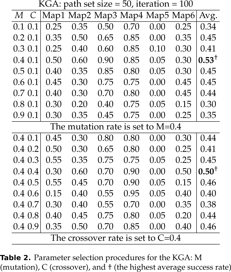
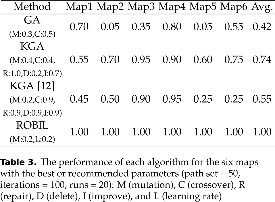
Table 3 shows the success rates of each algorithm when the best or recommended parameters were selected. In the first row, the mutation and crossover rates of the GA were set to 0.3 and 0.5, respectively. Similarly, the parameters for the KGA, mutation, crossover, repair, deletion and improvement rate were set to 0.4, 0.4, 1.0, 0.2 and 0.7, respectively. It is noteworthy that the experimental results of the success rates for each map, which are represented in the second and the third rows of Table 3, are obtained by using the same KGA [12]. Therefore, the difference between the success rates must derive from different KGA parameter settings. The KGA parameters in the second row of the first column are obtained by our parameter selection procedure; the KGA parameters in the third row of the first column are recommended by the authors [12]. Because the KGA parameters recommended by our parameter selection procedure yield superior success rates compared to the parameters recommended by the authors [12], in our experiments we set the KGA parameters according to the second row of the first column. From Table 3, we see that ROBIL demonstrates outstanding success rates even though the number of parameters used is much lower than in the KGA.
The performance of each algorithm for the six maps with the best or recommended parameters (path set = 50, iterations = 100, runs = 20): M (mutation), C (crossover), R (repair), D (delete), I (improve), and L (learning rate)
4.2. Success rate and robustness
The performance of an evolutionary algorithm can be significantly influenced by the size of the path set and the number of allowed iterations. Hence, we compared the success rates of the conventional GA, the KGA and ROBIL while changing these parameters. We also compared the variation in the success rates for each algorithm using a box-plot, and examined which algorithm showed stable performance despite changes in the number of path sets and iterations.
Figure 10 shows the success rate of each algorithm on the six maps when changing the size of the path set. Varying the size of the path set from 10 to 200, we observed the average success rate of 20 independent runs of each algorithm, with the number of allowed iterations fixed at 50. In Figures 10(a) and 10(b), we can see that the success rates of the conventional GA and KGA deviate widely, although they tend to increase with the size of the path set. Figure 10(c) shows that the proposed method outperforms both the GA and the KGA, and is more robust against the size of the path set.
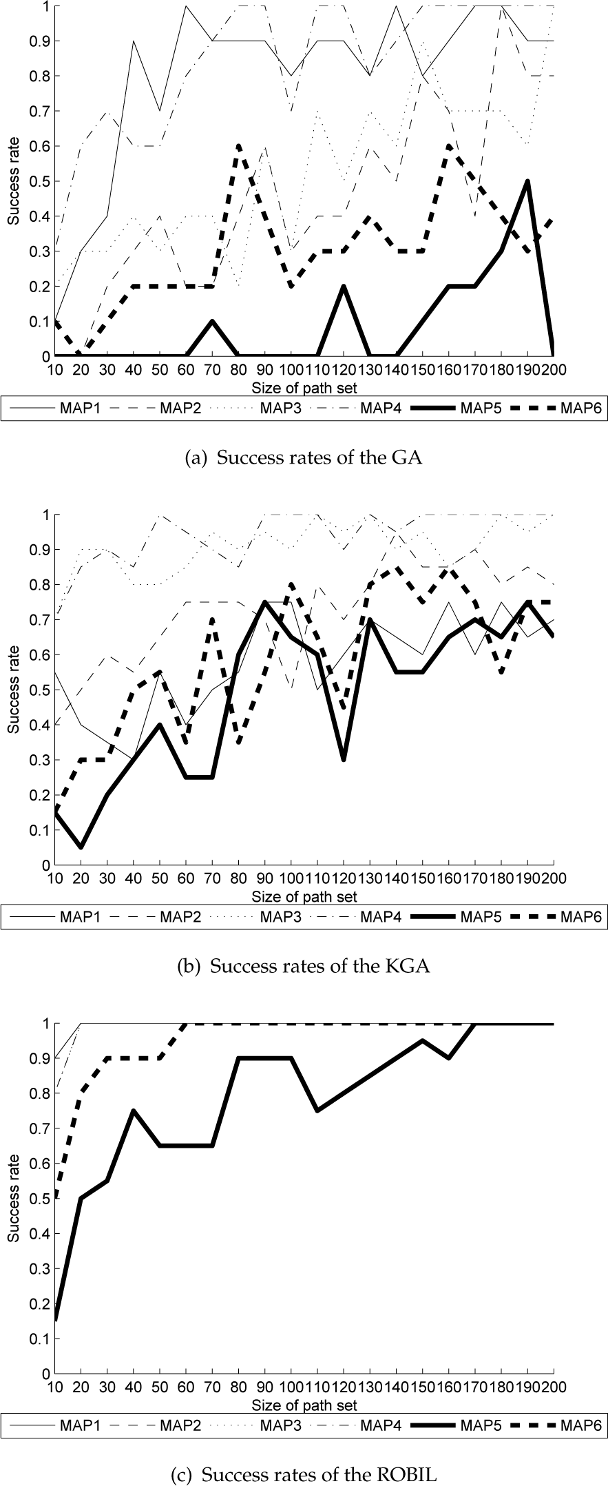
Success rates of the GA, KGA and ROBIL on six maps for different-sized path sets (path set = 10–200, iterations = 50, runs = 20)
We can see from Figure 10 that success rates are highly correlated with the size of the path set and that they tend to improve as the path set size increases. Therefore, we used a box-plot to examine more detailed performance statistics, when a path set size of more than 100 was set for each algorithm. The box-plot depicts groups of numerical data based on five elements: the smallest observation (lowest black bar), the lower quartile (base line of the box), the median (red bar), the upper quartile (topside of the box), and the largest observation (upper black bar). A red cross represents an outlier value. The box-plot also reveals the value distribution from the lower 25% to the upper 75% using the lower and upper quartiles. The median value represents the lower 50% position.
Figure 11 shows the box-plot of the success rates and their variances for each algorithm when a path set size of over 100 was set for each algorithm. In Figure 11(a), for example, the results of the GA on Map 2 show a maximum success rate of 1.0 and a minimum success rate of 0.3, as well as median, upper quartile and lower quartile values of 0.6, 0.8 and 0.4, respectively. From Figure 11(a), we can see that the GA has the lowest success rate and as well as highly unstable performance across all maps, despite sufficiently sized path sets. The results in Figure 11(b) indicate that the KGA provides a higher median, a lower quartile and an upper quartile than the GA. From Figure 11(c), we see that when the size of the path set was greater than 100, the success rate of ROBIL increased to 1 on Maps 1–4 and 6, and was also very high for Map 5. This indicates that the performance of ROBIL is both higher and more stable than the GA and the KGA.

Box-plot success rate distribution for each map and algorithm according to changes in the size of the path set (path set = 100–200)
Figure 12 shows the success rates when changing the number of iterations from 60 to 300 and fixing the size of the path set to 50. Figures 12(a) and 12(b) show that the conventional GA has the worst success rates and that these rates vary widely according to the number of allowed iterations, whereas the KGA provides generally higher and more stable success rates. However, Figure 12(c) shows that ROBIL had markedly better success rates and more stable performance than either the GA or the KGA when changing the number of allowed iterations.
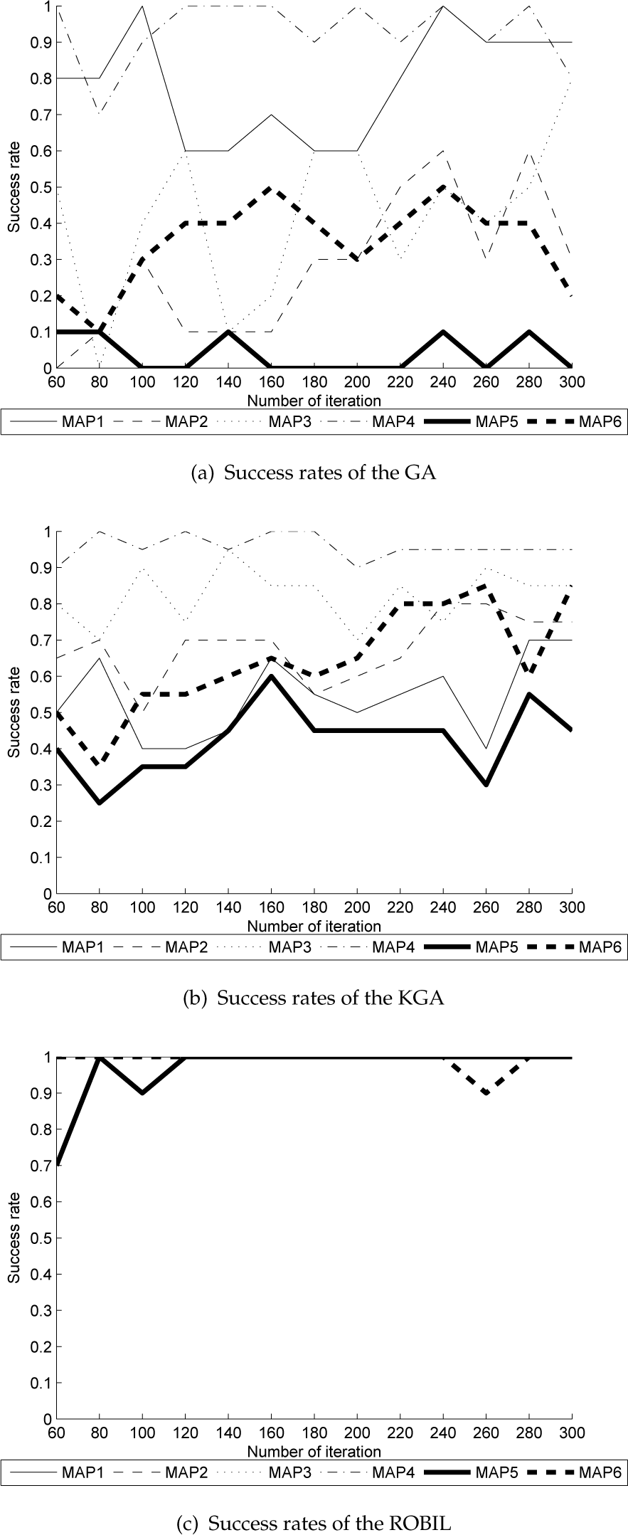
Success rates of the GA, KGA and ROBIL on six standard maps for different numbers of allowed iterations (path set = 50, iterations = 60–300, runs = 20)
4.3. Performance for shortest path planning
In this section, we validate the performance of the proposed ROBIL for shortest path planning in terms of the quality of the obtained path. Figure 13 shows the average distance of the path obtained by each algorithm on six maps when the size of the path set is more than 100, because a sufficient number of path sets is an important factor in obtaining feasible paths for each algorithm, as shown in Figures 10 and 12; the vertical axis represents the average distance of the obtained path, and the horizontal axis represents the size of the path set. Here, a lower average distance indicates a better quality path.

Comparison of average lengths of paths obtained by each algorithm according to the size of the path set (path set=100–200, iteration=50, runs=20)
In Figure 13, we can see that the overall quality of the obtained path improves with the size of the path set, and that ROBIL clearly outperforms both the conventional GA and the KGA. In Figure 13(a), we see that ROBIL finds better paths than the GA and the KGA regardless of the size of the path set. The average path lengths for the GA and the KGA gradually improve as the path set size increases. This tendency can be observed consistently in the five figures that follow 13(b)-13(f). It is interesting to note that we see the greatest difference in performance among the three algorithms in Map 5 and Map 6. This may result from the geometrical complexity of the given maps; the obstacles in Map 5, for example, are very close to one another, and most of the obstacles present dead ends. Overall, we conclude that ROBIL efficiently solves the path planning problem even for relatively complicated maps.
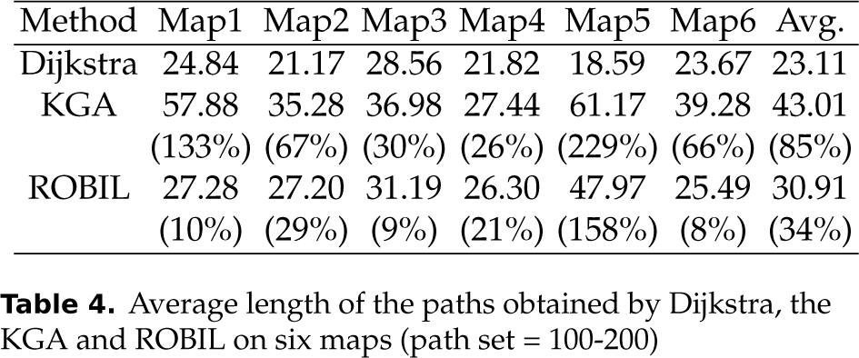
Table 4 lists the average lengths of the paths obtained for each map by Dijkstra, the KGA and ROBIL, and the performance ratio of ROBIL and the KGA over Dijkstra as a relative change in percentage. Dijkstra's algorithm is used to yield the optimal path and compare the quality of solutions. The average lengths of the paths on each map were calculated from the results in Figure 13, and the relative changes in percentage were calculated as the difference in the average length of the ROBIL and the KGA paths and the length of the Dijkstra paths, divided by the length of the Dijkstra paths. Note that in Table 4, we excluded the results for the GA. The GA consistently generated greater path lengths for all maps and sizes of path sets, as shown in Figure 13. From Table 4, we can see that the average length of the paths obtained by ROBIL was shorter than the average length of the paths obtained by KGA under all conditions. We can observe that the path length for ROBIL was 30% longer on average than the optimal path length for Dijkstra. The path length for the KGA was more than 85% longer on average than that for Dijkstra. Moreover, ROBIL tends to take much less time than the KGA. The average execution times for the KGA and ROBIL on the six maps were 24.5 s and 3.1 s, respectively; the average increase in speed that ROBIL achieved versus the KGA was eightfold. The experimental results indicate that ROBIL provide more efficient and effective paths than either the GA or the KGA. We represent the best path obtained by ROBIL in Figure 14.
Average length of the paths obtained by Dijkstra, the KGA and ROBIL on six maps (path set = 100–200)

The trajectory of the best path obtained by ROBIL on six maps (path set = 50, iteration = 50)
4.4. Performance for an unseen map
We examine the performance of ROBIL on an unseen map to verify that the parameters found from the six maps can be successfully used for an unseen map. Figure 15 shows a new map with a 16 × 16 grid that we label ‘Map 7’. This represents an office (indoor) environment. We set the number of allowed iterations to 50 and vary the size of the path set from 50 to 100. These parameters yielded good performances in most cases. The average distance of the obtained paths and the success rates are reported in Table 5.
Performance of ROBIL on Map 7 for path set = 50 and 100 (the optimal distance using Dijkstra's algorithm is 27.18)

A new, unseen map, that represents an office (indoor) environment, labelled ‘Map 7’
The experimental results indicate that ROBIL found a feasible path on Map 7 in 20 runs, because it achieved a success rate of 1.0. Therefore, we can state that the selected parameters can be successfully used on an unseen map. Moreover, we see that ROBIL found the near-optimal path because the difference between the average distance of the path obtained by ROBIL and the distance of the optimal path obtained by Dijkstra's algorithm is insignificant; the distance of the path obtained by Dijkstra algorithm is 27.18.
Additionally, we tested the performance of ROBIL on randomly created maps with different sizes; the sizes of these maps were 50 × 50, 100 × 100 and 150 × 150, respectively. Figure 16 represents the best path obtained by ROBIL on the three random maps. From the test results, it is observed that ROBIL found the feasible paths on randomly created maps all the time.

The trajectory of the best path obtained by ROBIL on three randomly created maps (path set = 50, iteration = 50)
4.5. Performance for the large-scale map
To test the scalability of ROBIL for large-scale maps, we performed additional experiments using the seven maps (Map 1-Map 7, Figures 8 and 15), where the size of each map was enlarged to a 200 × 200 grid. In our tests, a standard A* algorithm that uses the Euclidean distance using eight adjacent nodes as the heuristic function was employed to compare the quality of the solutions; it was compared to the other methods in terms of the average distance of the obtained path, the execution time in seconds, and the success rate. We excluded the experimental results of Dijkstra's algorithm from our tests because it became computationally prohibitive for these large maps (e.g., it took two days for Map 7). To obtain values in accordance with each criterion, we repeated each experiment 30 times, independently, and the average value was reported.
We compared the success rates of A*, the GA, the KGA and ROBIL for the seven large-scale maps in Table 6. It can be seen that the success rates of the A* algorithm and ROBIL were superior to those of the GA and the KGA. This represents a similar trend to the previous success rate experiments on the 16 × 16 maps in Section 4.2.
Comparison of success rates according to A*, the GA, the KGA and ROBIL (map size=200 × 200, path set=50, iteration=50, runs=30)

In Figure 17, the average execution times of A*, the KGA and ROBIL are presented. The experimental results indicate that ROBIL finds a feasible path in approximately 35 seconds regardless of the given map. It is interesting to note that the execution time of the A* algorithm is unstable, depending upon the given map. For example, the A* algorithm required 65 to 95 seconds to find a feasible path in Map 2, Map 3, Map 6 and Map 7. Consistently, ROBIL required 35 seconds. A possible reason for this may be found in the heuristic function of the A* algorithm. Because it is difficult to determine which heuristic function is suitable to what map, the A* algorithm may search the path inefficiently according to the structure formed by the obstacles on the given map. Of the three methods, the KGA gave an extremely inefficient overall performance.

Comparison of the execution time in seconds for obtaining a path according to A*, the KGA and ROBIL (map size=200 × 200, path set=50, iteration=50, runs=30)
In Figure 18, the average distance of the A* algorithm and ROBIL, according to the seven maps, is shown. Overall, the A* algorithm provided slightly shorter distances than ROBIL. In contrast, we found that ROBIL calculated a shorter path than the A* algorithm for Map 7. For further analysis, we plotted the trajectories of the best paths obtained by Dijkstra's algorithm, the A* algorithm and ROBIL in Figure 19. Figure 19(a) shows the optimal path obtained by Dijkstra's algorithm; the length of the optimal path is 354. Figure 19(b) indicates that the trajectories of the path obtained by the A* algorithm were formed to take a longer route (the path length is 372) because the A* algorithm considers eight adjacent nodes in each searching process. Figure 19(c) shows the path when the A* algorithm considers all reachable nodes as the neighbours of a node; although it found the optimal path (the path length is 354), it took two days to do so due to the high computational cost. Figure 19(d) shows that the trajectories of the best ROBIL path are a better solution (the path length is 356) by discarding the unnecessary passage nodes visited in the A* algorithm. From the test results, we see that ROBIL gives a competitive performance in comparison to the A* algorithm for most cases in terms of execution time and path distance.

Comparison of the average distance of paths according to A* and ROBIL (map size=200 × 200, path set=50, iteration=50, runs=30)
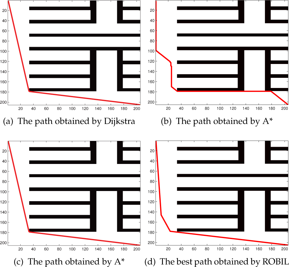
(a) The trajectory of the best path obtained by Dijkstra's algorithm; (b) the A* algorithm considering eight adjacent neighbours, (c) the A* algorithm considering all reachable neighbours, and (d) ROBIL, all on Map 7 (path set = 50, iteration = 50)
5. Conclusion
We described and demonstrated our ROBIL algorithm for an efficient solution to mobile robot path planning problems, and confirmed that ROBIL can reliably find a near-optimal path using a small number of parameters. To verify the potential of ROBIL, we compared it to two well-known evolutionary algorithms: a conventional GA and a KGA. The conventional GA demonstrated very low success rates and unstable performance for the parameters used, while the KGA's use of additional operators (e.g., repair, delete and refine) gave it certain performance advantages but also created greater computational complexity and parameter sensitivity, leaving its performance unstable. In contrast, ROBIL provided a considerably high success rate and stable performance, despite using far fewer parameters than the KGA. Furthermore, from a series of experiments on large-scale maps, we found that the proposed ROBIL has the potential to provide scalability to large-scale maps; it is superior and competitive compared to well-known conventional methods, such as the A* algorithm.
Having focused in this study on developing an effective algorithm with near-optimal parameters, we leave to future work the development of effective hybrids of the ROBIL algorithm and an exploration of the differences in initial population quality. Issues involved in reducing the convergence time by improving the probability model and decreasing the space complexity required for storing the edge bank are also left for future work.
Footnotes
6. Acknowledgements
This work was supported by a National Research Foundation of Korea Grant funded by the Korean Government (No. 2012R1A1A1001969) and by the Kyungpook National University Research Fund, 2012.