
Abstract
The ability to estimate Cartesian space trajectories that include orientation is of great importance for many practical applications. While it is becoming easier to acquire trajectory data by computer vision methods, data measured by general-purpose vision or depth sensors are often rather noisy. Appropriate smoothing methods are thus needed in order to reconstruct smooth Cartesian space trajectories given noisy measurements. In this paper, we propose an optimality criterion for the problem of the smooth estimation of Cartesian space trajectories that include the end-effector orientation. Based on this criterion, we develop an optimization method for trajectory estimation which takes into account the special properties of the orientation space, which we represent by unit quaternions. The efficiency of the developed approach is discussed and experimental results are presented.
1. Introduction
The estimation of human hand motion is an important problem for many applications. Our interest stems from programming by demonstration [1] (also called ‘imitation learning’) in robotics. Figure 1 shows an example of a programming by demonstration system where a robot is guided to perform a classic peg-in-hole task [2]. The goal of imitation learning is to provide robotic systems with the ability to relate perceived human actions to their own embodiment in order to learn - and later perform - the demonstrated actions [3]. In imitation learning, knowledge about the demonstrated human hand motion is often essential for the understanding of the demonstrated behaviour.

Demonstration of a peg-in-hole operation. The human demonstrator observes the performance of the robot and adapts his hand motion so that the robot successfully executes the task. The demonstrator's hand motion is measured by Kinect.
Ignoring the fingers, we normally encode hand motion as a rigid body motion. It is well known that rigid body motion consists of a translational and a rotational part [4]. The reconstruction of a pure translational motion can be accomplished by standard optimization methods, because the set of all translations forms a three-dimensional (3D) vector space. On the other hand, the set of all rotations in the 3D Cartesian space, which we denote by SO(3), forms only a group and not a vector space. The special Euclidean group SE(3) is defined as a semi-direct product of ℝ3 and SO(3). It represents the Euclidean transformation of rotation followed by translation. Unfortunately, there exists no representational scheme for rotations that would be simultaneously non-redundant, continuous and free of singularities [4]. This causes problems when solving optimization problems for SO(3) because representations free of singularities (e.g., rotation matrices and quaternions) contain more than the minimal number of parameters. The resulting parameters are therefore not independent of each other.
One possibility for measuring human arm and hand motion is to use RGB-D sensors, e.g., Kinect. The Kinect sensor uses the principle of structured light and captures depth and colour images simultaneously at a frame rate of about 30 Hz [5]. Together with the appropriate software, Kinect enables the tracking of several joints on the human body, including hand position and orientation [6, 7]. No special markers are needed. This results in a sequence of noisy measurements of the form:

The problem of smoothing on general Riemannian manifolds has been considered in general mathematical texts [18–20]. The approach proposed in this paper is a special case of smoothing on Riemannian manifolds. Unlike these more general papers, in this paper we focus on a specific problem of smoothing in ℝ3 × S3 and address many particular issues relevant to this problem, e.g., the definition of tangential space and metrics using an exponential and logarithmic map and how to use them within the framework of the Gauss-Newton and Levenberg-Marquardt methods on R3 × S3.
As mentioned above, SO(3) cannot be globally embedded in the 3D Euclidean space. This means that if the rotation group is represented by three real parameters (e.g., as in the case of Euler angles), the Euclidean metric topology in ℝ3 does not induce a global topology or metric structure in SO(3). This is the main motivation for selecting unit quaternions to represent rotations - the spherical metric of S3 corresponds to the angular metric of SO(3) [21]. We would, however, obtain similar results if we used a different representation free of singularities, e.g., rotation matrices. In the following, we first formulate the problem of estimating motion trajectories on ℝ3 × S3 and then propose an optimization method that can be applied to solve it. The main feature of our approach is that we exploit the properties of the exponential map to calculate new estimates at each step of the iterative optimization process, which enables us to formulate the optimization process directly on ℝ3 × S3.
2. Preliminaries
Formally, a quaternion q = (w, u1, u2, u3) is a vector quantity, where w is the scalar component of q and u = [u1,u2, u3]T is the vector component. The quaternion multiplication is defined by:

Quaternions form a non-commutative group with respect to the above multiplication. The magnitude of a quaternion is defined as:


where ̄ is the conjugate of q. Given a rotation by V about a unit axis vector n, we define the associated unit quaternion as:

There is a 2-1 mapping between unit quaternions and the rotation group [21]. Each rotation from SO(3) can thus be represented by two quaternions belonging to the unit sphere S3 ℝ4. However, the two unit quaternions representing the same rotation are well separated because they lie on different sides of the unit sphere. It can be shown that a vector v′ ∈ ℝ3, rotated from a vector v ∈ ℝ3 by a rotation represented by a unit quaternion q, can be calculated by a simple quaternion multiplication:

In this multiplication, the 3D vector v is treated as a quaternion with a zero scalar component. It is easy to see that the resulting quaternion v′ has a zero scalar component as well.
In the following, we will need the exponential map exp : ℝ3 ŕ S3, which is given by:
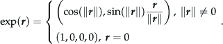
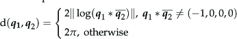
We denote by T q (S3) C ℝ4 the tangent space of S3 at unit quaternion q. It can be shown that the exponential map transforms a tangent vector r ∈ T1 (S3) = ℝ3 into q ∈ S3, where q is a quaternion at distance ||r|| from the identity quaternion 1 (a unit quaternion with a zero vector component) along the geodesic curve, which is given by q(t) = exp(t log(q)), starting from quaternion 1 in the direction of r. The geodesic curve represents the shortest path from 1 to q on S3. The logarithmic map log : S3 → ℝ3 is defined as:

If we limit the domain of the exponential map to ||r|| < π and the domain of the logarithmic map to S3/(– 1,0,0,0), then both mappings become one-to-one, continuously differentiable and inverse to each other. It can be shown that the expression:
3. Formulation of the Problem
The estimation of noisy vector-valued measurements with non-diagonal covariance matrices has been considered by [22, 23], who developed an iterative algorithm for the nonlinear estimation of a smooth vector-valued function based on a non-parametric optimality criterion. In our case, the problem is more complicated because the space of all orientations is not a vector space. While the difference between the measured and the true position can be modelled as additive, namely:


We assume that the error in the position and orientation is Gaussian with zero mean and a covariance matrixσ k . The changing of the current position P1k and orientation q1k by a deterministic displacement (ΔPk, Δqk) results in:

We note that the position error vector remains unchanged under transformation (12). To find the relationship between the old and the transformed rotation error vector, we make the following observation:

Hence, there exists the following relationship between the two error vectors:


The new error vector is obtained by rotating the old error vector into a new orientation. Writing the covariance matrix σ
k
as:


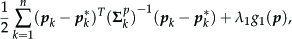
The aim of reconstruction is to find a trajectory that not only approximates the measurements well but is also smooth. If the measurements were simply interpolated, the reconstructed trajectory would not be smooth enough. Hence, we must search for a compromise between smoothness and goodness of fit. Writing P = [pT1,…,pTn and q = [qT1,…, qTn]
T
, the goodness of fit can be evaluated by:

A good measure of the smoothness of trajectories is given by the amount of linear and angular acceleration. The linear acceleration ak, k = 2,…, n – 1, can be estimated by:
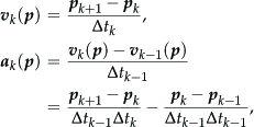
where Δtk = tk+1 – tk. Similarly the angular acceleration αk, k = 2,…, n – 1, can be estimated by:

Writing:
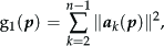

we can formulate the following criterion, which should be minimized by a rigid body motion that exhibits good balance between smoothness and goodness of fit:
The parameters λ1 and λ2 govern the trade-off between the two criteria.
Since the criterion function (20) is nonlinear, we must apply nonlinear optimization techniques to find the optimal sequence of poses (Pk, qk). The minimization of (20) over pk, qk would be a classic nonlinear least squares optimization problem if we could treat unit quaternions qk as elements of ℝ4 and not of S3. Since this is not the case, the classic approach would be to add the constraints qk = 1 to the optimization criterion. However, such constraints make the optimization problem significantly harder. In the following, we propose a technique that can be used to optimize the criterion (20) without specifying additional constraints.
4. Optimization in ℝ3 × S3 × … × ℝ3 × S3
The tangent space T
q
(S3) C ℝ4 is defined as a space that contains the directions of all paths on S3 passing through the quaternion q. As mentioned in Section 2, the exponential map exp transforms a tangent vector r ∈ T1(S3) = ℝ3 into a point

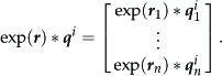
It can be shown [24] that x * ̄ ∈ T1 (S3) or - in other words - x * ̄ is a quaternion with a zero scalar component, for anyx ∈ T q (S3), q ∈ S3. Thus, the above mapping is well-defined for all x ∈ T q (S3). As the mapping x * ̄ is an isomorphism from T q (S3) to ℝ3, all the unit quaternions in the neighbourhood of q can be represented by exp(r) * q, r ∈ ℝ3.
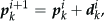
Taking (pik, qik) ∈ ℝ3 × S3, k = 1,…n, to be the i-th estimate for the optimal sequence of positions and orientations, it is appropriate to calculate the next sequence of positions and orientations as follows:

where:
The above criterion can be rewritten as:

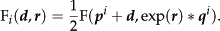
where:

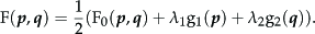
is a vector function from ℝ 6n to ℝ12n–12. The gradient and the Hessian of Fi are given by:

where Ji(d, r) is the Jacobian of f at (d, r) and k i are the component functions of fi.
The Taylor series expansion for the vector function ▿F i around ▿F i (0,0) is given by:

If we assume that the value of F
i
is small for all q belonging to the neighbourhood of the solution (i.e., fki(d, r) ≈ 0 for all k), we obtain from Eq. (27) the following approximation for the Hessian in the neighbourhood of the solution:

The next sequence of poses can then be calculated using Eq. (22) and (23). The iteration is stopped when:

Note that JTi Ji ∈ ℝ6nx6n is a symmetric band matrix with bandwidth 35 (17+1+17). Thus, the number of arithmetic operations needed to solve the resulting linear system of equations is linear with respect to the number of measurements. Note that this is by far the most computationally expensive part of our system. Since we have a good initial approximation for our optimization problem (the measurements themselves are used to initialize optimization), there are not too many iterations that need to be performed in order to find the optimal solution (see also Table 1). Hence, our approach can easily deal with thousands of measurements, which is the order of magnitude for the number of data points we normally acquire when measuring demonstrated trajectories. Demonstrated trajectories are usually acquired at 30 Hz, and up to 120 Hz with marker-based systems, and take from a few seconds to tens of seconds. Note also that batch optimization is by definition offline; hence, real-time operation is not an issue.
Convergence of the Gauss-Newton method for different smoothing parameters.
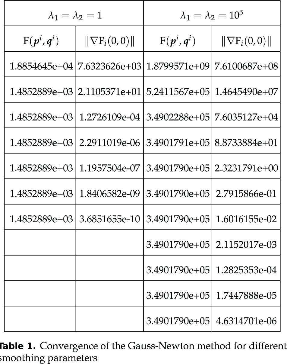
The counterpart of the derived iteration in real spaces is the Gauss-Newton iteration. Actually, we have shown above how to carry out the Gauss-Newton iteration on ℝ3 × S3 × … × ℝ3 × S3. However, the classic Gauss-Newton method can encounter problems when the second-order term in Eq. (27) is significant. While for small smoothing parameters λ1, λ2 the criterion functions fki are also small in the neighbourhood of the minimum, this is not the case for larger smoothing parameters. Therefore, we can expect slower convergence when the smoothing parameter becomes large.
We can overcome this problem by applying the Levenberg-Marquardt method, in which the search direction is calculated as follows:

Note that the system matrix (JTiJi + μiI) is positive definite for every μi > 0. When μi is equal to zero, the search direction becomes identical to that of the Gauss-Newton method. As μi tends towards infinity, (di, ri) tends towards a vector of zeros and a steepest descent direction. This implies that, for some sufficiently large μi, the value F i (di, ri) is smaller than F i (0,0) = F(pi, qi). Thus, the Levenberg-Marquardt method uses a search direction that is a cross between the Gauss-Newton direction and the steepest descent.
It remains to show how to determine the smoothing parameters λ1 and λ2. It is important to properly select the degree of smoothing to find a proper balance between smoothness and goodness of fit. Often, methods like cross-validation are used, but in general cross-validation is computationally expensive because it requires that the data be partitioned into two sets: one used to learn or train a model, and the other used to validate the model. These sets need to be changed many times so that all the data can be validated. For this reason, we prefer to use an approach proposed in [25] for the case when the amount of noise associated with the data is known. With this method, we can determine the optimal values for λ1 and λ2 by solving the following nonlinear systems of equations:


Unlike in (20), where the calculation of Pk,qk is coupled through the covariance matrices, here, the smoothed positions and orientations Pk (λ1), qk (λ2) are calculated in a decoupled way by solving:

Assuming that σ
p
k
and σ
q
k
are the covariance matrices of the measurements, the acceptable values for S1 and S2 are within the range
The described method finds a smooth sequence of hand postures that approximate the measurements well. To generate a continuous motion trajectory that can be used for robot control, one must interpolate the smoothed postures. While standard techniques for interpolation in ℝ n [26] can be utilized for the interpolation of position vectors, more specialized methods are needed for smooth interpolation on SO(3). The most commonly used quaternion interpolation method is spherical linear interpolation (Slerp), proposed by [21], but more advanced methods that can ensure higher-order smoothness also exist [27].
5. Experimental Results and Conclusions
We applied the developed method for the reconstruction of 15 real hand motions. In these experiments, the Gauss-Newton method always converged. As expected, the convergence was slower for larger values of smoothing parameters (see Tab. 1). The measured poses were used as a starting point in iteration (30) or (32). One example smoothed trajectory, which was calculated at the optimal values of the smoothing parameters, is depicted in Figures 2, 3 and 4. In this way, smoother trajectories were estimated that resulted in less jerky robot movements.

The translational part (x, y and z components) of the reconstructed trajectory (in centimetres) and a sample of measurements. Not all measurements are shown for better visualization.

The orientational part (x, y andz components of u(t), q(t) = (w(t), u(t))) of the reconstructed trajectory and a sample of measurements. Not all measurements are shown for better visualization.

The orientational part (w component of q(t) = (w(t),u(t))) of the reconstructed trajectory and a sample of measurements. Not all measurements are shown for better visualization.
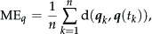
To show the benefit of the proposed approach, which considers full covariance matrices σ k and computes positions and orientations simultaneously, we compared it to scalar spline smoothing, where each component is evaluated separately. Decoupled smoothing of separate components of unit quaternions has an additional disadvantage that the smoothed quaternions are not unit quaternions. They should, therefore, be normalized after smoothing, which introduces additional errors. Note that scalar spline smoothing also requires the determination of an optimal smoothing parameter λ. The comparison was done in a simulation experiment where the correct position p(t) ∈ ℝ3 and orientation trajectories q(t) ∈ S3 were known. To the simulated trajectories, we added Gaussian noise using preselected covariance matrices σ k . The quality of approximation was evaluated using the mean error, namely:

where d is the metric on S3 defined in Eq. (9). Results for a typical trajectory are shown in Tab. 2. Significant improvement could be achieved both in position and the orientation trajectory.
In summary, in this paper we developed two trajectory estimation methods on ℝ3 × S3 - one based on Gauss-Newton iteration and the other on Levenberg-Marquardt iteration. We have also shown how to treat the measurement errors and suggested an approach for the automatic calculation of smoothing parameters. The method based on Gauss-Newton iteration turned out to be sufficient in our experiments and converged faster. However, it might become necessary to apply the method based on Levenberg-Marquardt iteration for the data containing more noise. With our approach, we were able to reconstruct smooth trajectories on ℝ3 × S3 using real data obtained by measurement systems with or without markers. In this way, we can provide a high quality input for imitation learning systems.
Comparison of smoothing with the proposed approach and with scalar spline smoothing, where each position and quaternion dimension is smoothed separately.

Footnotes
6. Acknowledgments
This research has received funding from the European Community's Seventh Framework Programme FP7/2007-2013 (Specific Programme Cooperation, Theme 3, Information and Communication Technologies) under grant agreement no. 600578, ACAT.