Sage Journals: Discover world-class research

Abstract

In this research, adaptive perception for driving automation is discussed so as to enable a vehicle to automatically detect driveable areas and obstacles in the scene. It is especially designed for outdoor contexts where conventional perception systems that rely on a priori knowledge of the terrain's geometric properties, appearance properties, or both, is prone to fail, due to the variability in the terrain properties and environmental conditions. In contrast, the proposed framework uses a self-learning approach to build a model of the ground class that is continuously adjusted online to reflect the latest ground appearance. The system also features high flexibility, as it can work using a single sensor modality or a multi-sensor combination. In the context of this research, different embodiments have been demonstrated using range data coming from either a radar or a stereo camera, and adopting self-supervised strategies where monocular vision is automatically trained by radar or stereo vision. A comprehensive set of experimental results, obtained with different ground vehicles operating in the field, are presented to validate and assess the performance of the system.

Keywords

Driving Automation Robotics Vehicles Adaptive Learning Multi-sensor Perception

1. Introduction

The latest research and industrial efforts in the automotive field have been devoted to increase the degree of autonomy towards the ultimate goal of fully driverless vehicles. In this respect, traversable ground detection continues to represent an open issue that needs to be addressed. This is especially true in outdoor settings, where conventional perception systems that assume flat ground or else use roadway markings would lead to failure, as the terrain typically exhibits widely-varying geometric (i.e., size and shape) and appearance (i.e., texture and colour) properties, due to the presence of slopes and holes, different vegetation types, and changes in the illumination conditions or weather phenomena, including rain and snow. One possible solution for reliable long-term classification is the use of online learning strategies.

In this work, an adaptive statistical framework is proposed for automatic terrain estimation. Typically, it comprises two stages: a training stage and a classification stage. In the training stage, the system automatically learns to associate salient features that are extracted from sensor data with the ground class. Next, it is able to label new observations based on past data. A one-class classification approach is adopted where only the ground class is defined and modelled using a mixture of Gaussians (MoG). New observations are labelled using an outlier rejection strategy based on their Mahalanobis distance from the ground model.

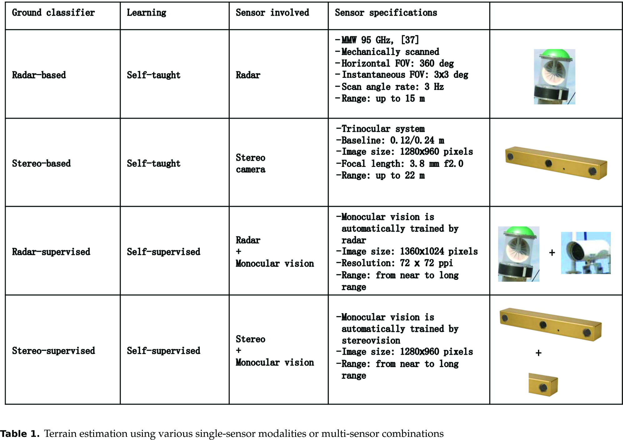
The system features modularity and single classifiers based on different sensor data can be used in cascade to form a self-supervised system whereby one algorithm provides automatic training examples to the second algorithm. Following this rationale, distinct embodiments of the same self-learning scheme are presented: two self-taught classifiers using radar and stereo data, respectively, and two self-supervised algorithms where a monocular visual classifier is trained by either radar or stereo vision. Table 1 summarizes the properties of the different classifiers along with the main technical specifications of the sensors involved.

Table 1.

Terrain estimation using various single-sensor modalities or multi-sensor combinations

Ground classifier	Learning	Sensor involved	Sensor specifications
Radar–based	Self-taught	Radar	–MMW 95 GHz, [37]–Mechanically scanned –Horizontal FOV: 360 deg–Instantaneous FOV: 3×3 deg–Scan angle rate: 3 Hz –Range: up to 15 m
Stereo–based	Self–taught	Stereo camera	–Trinocular system–Baseline: 0.12/0.24 m–Image size: 1280×960 pixels–Focal length: 3.8 mm f2.0–Range: up to 22 m
Radar–supervised	Self-supervised	Radar + Monocular vision	–Monocular vision is automatically trained by radar–Image size: 1360×1024 pixels–Resolution: 72 × 72 ppi–Range: from near to long range
Stereo–supervised	Self–supervised	Stereo + Monocular vision	–Monocular vision is automatically trained by stereovision–Image size: 1280×960 pixels–Range: from near to long range

One important aspect of the proposed framework is that the ground model is recursively updated during vehicle operation using the latest sensor data, thus making it feasible for long-range and long-duration perception over changing environments. In summary, the following main advantages can be derived: (a) an adaptive online ground modelling approach that makes the system feasible in long-range and long-duration applications; (b) a unified self-learning framework for ground detection that can be applied using a single sensor or else by combining different sensor modalities; (c) self-supervised visual classification to extend the region of inference from the near range to the far range, and to provide rich 3D environment mapping by combining range and appearance information; (d) the use of a MoG for the detection of multiple terrain components within the broad class of the ground.

The proposed classifiers have been extensively tested in the field using two test beds, i.e., an all-terrain robot and an agricultural tractor, demonstrating their effectiveness in different environments and conditions.

The paper is organized as follows. Section 2 surveys the related research. Section 3 details the self-learning framework. In Section 4, the statistical classification strategy is described. Section 5 details the single and multi-sensor implementations, providing experimental results attesting to the feasibility of this approach. Conclusions and future developments are drawn in the final Section 6.

2. Literature review

Terrain surface detection and classification is an important task to increase the degree of automation of intelligent vehicles towards the ultimate goal of fully driverless vehicles. Many approaches have been proposed in the literature, using different ground models and sensor combinations. Ground detection algorithms can be classified into deterministic (no learning), supervised and self-supervised algorithms. Under deterministic approaches (e.g., [1], [2], [3]), terrain features such as slope, roughness and discontinuities are analysed to segment the traversable regions from the obstacles. Some visual cues, such as colour, shape and height above the ground have also been employed for segmentation in [4], [5]. However, these methods assume that the characteristics of obstacles and of the traversable ground are fixed, and therefore they are not suited to rapidly changing environments. Without learning, such systems are constrained to a limited range of predefined settings.

Supervised learning approaches have been proposed, especially in the automotive field and for structured environments (e.g., in road-following applications). These include ALVINN (Autonomous Land Vehicle in a Neural Network) by Pomerlau [6], MANIAC (Multiple ALVINN Network In Autonomous Control) by Jochem et al. [5], and the system proposed by LeCun et al. [7]. ALVINN trained a neural network to follow roads and was successfully tested at highway speeds in light traffic. MANIAC was also a neural net-based road-following navigation system. LeCun et al. used end-to-end learning to map visual input to steering angles, producing a system that could avoid obstacles in off-road settings but which did not have the capability to navigate to a goal or map its surroundings. Many other systems have been proposed recently based on supervised classification strategies [8], [9], [10]. For instance, in [10], laser range, colour and texture cues are combined to segment dirt, gravel and asphalt roads by training separate neural networks on labelled feature vectors clustered by road types. These systems were manually trained offline, and therefore the scope of their expertise is limited to environments seen during training. In order to solve this issue, Dima et al. [11] proposed active learning to limit the amount of labelled data in a mobile robot navigation system. Only recently, self-supervised systems have been introduced to reduce or remove the need for hand-labelled training data, thus gaining flexibility in unknown environments.

Self-supervised approaches exploit a reliable classification module to provide input labels for the training of another classifier. Typically, a classifier producing reliable results at short range serves as the supervising module and is used to train a second classifier that operates on more distant scenes, thus providing a near-to-far range classification system. The bootstrapping of the supervising module is performed by manual training or by using some constraint on the ground geometry. For instance, in [12], two proprioceptive short-range terrain classifiers, one based on wheel vibration and one based on traction force, are used to train an exteroceptive vision-based classifier that identifies instances of terrain classes at long range. Both supervising modules rely on a priori knowledge of the terrain classes in the environment and use either hand-labelled training data or predefined thresholds, thus solving only in part the self-supervision problem. In [13], data from a stereo camera are used to train a monocular image classifier that segments the scene into obstacles and ground patches within a sub-modular Markov random field (MRF) framework. In detail, first, the largest planar region in the stereo disparity image is detected using a robust least squares procedure. Next, short-range classification is used as input to the learning algorithm for MRF-based classification at long-range.

LIDAR sensors have been proved successful for supervision in several works. In [14], a laser scanner is employed to supervise a monocular camera. Specifically, the laser scans for flat terrain in front of the vehicle by looking for height differences within and across map cells and modelling point uncertainties in a temporal Markov chain. Afterwards, the detected area is projected in the camera image and is used as training data for a vision algorithm that learns online a visual model of the road. In [15], a LIDAR-based manually trained SVM classifier is employed as the supervising module for a visual classifier to detect the ground in forested environments.

Although vision and LIDAR generally provide useful features for scene classification [16], they are both affected by weather phenomena or other environmental factors, such as smoke and dust [17]. Some LIDARs exist that partially solve this issue by sensing the ‘last echo’ return, but they also fail when the obscurant reaches a sufficient density. Cameras are also highly affected by lighting conditions and are unsuccessful in the presence of airborne obscurants. In contrast, millimetre wave radar penetrates dust and other visual obscurants, and detect distributed and multiple targets that appear in a single observation, whereas LIDAR systems are generally limited to one target return per emission (although multi-peak and last peak-based lasers address this issue to some extent and are becoming more common). Radar's persistence to low visibility conditions was investigated in numerous papers, for example in [17] and [18]. Nevertheless, radar has shortcomings as well, due to specularity and multipath effects that result in data ambiguities as well as difficulties in mapping and classification tasks. Therefore, to expand its range of applicability, radar can be combined with other sensors. Video sensors lend themselves very well to this scope since, in good visibility conditions, they generally supply a high resolution within a suitable range of distances and provide several useful features for the classification of different objects present in the scene [19], [20], [21]. Due to the complementary characteristics of radar and vision, it is reasonable to combine them in order to get improved performance.

Radar and vision fusion has been discussed mostly for in-road applications [22], [23], [24], [25], [26]. For instance, in [22] radar and vision independently detect targets of interest and then a high-level fusion approach is adopted to validate the radar targets based on visual data. A radar-vision fusion method for object classification into the category of ‘vehicle or non-vehicle’ is developed in [23]. It uses radar data to select visual attention windows, which are then assigned a label and processed to extract features to train a multi-layer in-place learning network (MILN). In [24], a vehicle detection system that combines radar and vision data is introduced. First, radar data are used to locate areas of interest on images. Next, a vehicle search is performed in these areas mainly based on vertical symmetry. A guard rail detection approach and a method to manage overlapping areas are also developed to speed up and improve the performance of the system. The combination of a fixed radar sensor with vision through sensor-fusion techniques has been successfully demonstrated at the DARPA Urban Challenge [26]. However, in this approach, a forward-facing radar system was specifically tuned for vehicle detection with a narrow horizontal field of view of only 15 deg. The sensor was mainly used for the position and velocity estimation of vehicles and obstacles directly ahead rather than for general scene classification.

Research on radar-vision combination has been presented by the authors in previous work. First, an expert rule-based radar ground detection method was developed to supervise a visual classifier in [27] and [28]. The latter algorithm employed a one-class classification strategy based on a single Gaussian model of the ground to segment each incoming video frame into ground and non-ground regions. However, the use of a uni-modal Gaussian model may not be sufficiently accurate in the presence of multiple terrain types. A machine learning approach to improve radar classification was introduced by the authors in [29]. Specifically, a self-trained radar classifier was developed where the ground model was learnt during a bootstrapping stage and recursively updated using the most recent ground labels to predict ground instances in successive scans. In [30], the same radar classifier served as the supervising module for a visual classifier. Both classifiers adopted a self-learning framework which can be considered of general applicability independently of the type of sensor used. In order to account for multi-modality in the feature data set distribution, a MoG was used to model the ground appearance, thus also allowing for the detection of terrain subclasses in addition to the ground segmentation task. The use of MoGs for visual ground modelling has been previously demonstrated in the literature (see, for instance, [14]); however, here a different method is developed in which both the modes and the number of components of the MoG are estimated online using an EM-BIC algorithm, and this is applied to two sensor modalities (i.e., radar and monocular vision). A similar classification framework was also successfully demonstrated by the authors using data from a stereo vision device in [31]. This paper reviews research by the authors in the context of self-supervised ground detection using different sensor combinations.

3. Adaptive self-learning

In this work, ‘self-learning’ will refer to the automatic training of a classification algorithm. One can generate the training set either via a self-teaching approach, where the classifier uses its own predictions to teach itself (i.e., self-taught learning), or using the output of another classification module (i.e., self-supervised learning) [32]. Either way, whether self-taught or self-supervised, the training set is not fixed and is continuously updated as new sensor data are gathered and classified during the robot's motion. Adaptive self-learning methods remove the need for manually labelled training data, thus gaining flexibility in unknown environments through the ability to adapt to changing environments on-the-fly.

In the case of a single sensor classifier (or a self-taught classifier), an initialization or bootstrapping stage is required where the vehicle starts its operation from an area free of obstacles in the sensors' fields of view. This ensures that the system initially looks at the ground only. Next, features can be extracted from sensor data and associated with the ground class. Following this strategy, the system learns the appearance of sensor data pertaining to the ground class and it can predict the presence of the ground in successive scans based on past knowledge.

In addition, assuming that a range sensor is employed, the single sensor classifier can be used to train a visual classification module that performs pixel-based segmentation of the image into ground and non-ground regions. Specifically, the first algorithm will survey for a drivable surface within the vicinity of the vehicle. These ground-labelled points are projected onto the visual image and used to set interest windows from which visual features can be extracted to build a visual model of the ground. In addition to the ground segmentation task, the visual classifier can also discriminate between different terrain components within the broad class of the ground. Thus, the two modules work in cascade, featuring a self-supervised learning scheme able to perform image segmentation and detect the different local components of the ground.

4. Statistical ground classification

Ground modelling is expressed as a one-class problem [33]. One-class classification methods are generally useful in two-class classification problems, where one class (the target class) is well-sampled while the other class (the outlier class) is under-sampled or else is not easy to model. The goal of a one class-classifier is that of building a decision boundary that separates the target class from all other possible objects. In our application field, ground samples are the target class while non-ground samples (i.e., obstacles) are considered as the outlier class. For outdoor environments, non-ground samples are typically sparse and the variation of all possible non-ground classes is virtually unlimited, thus making the non-ground class difficult to model. Conversely, the ground class is generally less variable, although it may change geographically and over time. Therefore, the problem can be reasonably formulated as a distribution modelling problem, where the appearance of the ground is the distribution to estimate.

4.1. Ground model

For ground modelling, a MoG is adopted, with each component describing a local terrain component. In the literature, MoG models have been demonstrated to be effective for clustering, since they allow each cluster to be represented in a compact form based on three main parameters: the mean vector, the covariance matrix and the number of members of the cluster. The parameters of a MoG can be obtained using expectation maximization (EM), although it requires a priori knowledge of the number of components K of the Gaussian mixture. The choice of the optimal number of Gaussian components is a critical issue, especially in online estimation problems, such as terrain modelling. On the one hand, a small number of components may be not enough to identify non-homogeneous ground regions; on the other hand, a high value of K could lead to over-fitting problems with a loss of generalizability for the classifier. In addition, knowledge of K would entail the number of habitats to be known prior to training, which is not generally the case for autonomous navigation.

In this research, EM and a Bayesian information criterion (BIC) are used to fit the data using a MoG model and estimate - at the same time - the optimal number of Gaussian components. Specifically, the optimal MoG model is found using a recursive procedure that starts with a single component assumption and iteratively applies EM with an increasing number of components up to a predefined maximum value. Eventually, the best-fitting model is chosen as the one that leads to the smallest value of the BIC statistic. The BIC balances the likelihood increase due to the number of parameters by introducing a penalty term that grows with K. Thus, two models can be compared, with the model with the smaller value of the BIC statistic being preferred [34].

It is worth noting that in order to account for ground changes during vehicle travel, the EM-BIC MoG fitting algorithm is applied on a frame-by-frame basis such that the ground model is recomputed based on the most recent ground-labelled observations.

4.2. Sensor data labelling

Given a new observation, i.e., a feature vector that will be set according to the type of sensor used (see Section 5.1.1 for radar, Section 5.2.1 for stereo vision and Section 5.3.1 for monocular vision), the classification step aims to assess whether this observation is an instance of the ground. A Mahalanobis distance-based approach is adopted, in which the Mahalanobis distance and its distribution are employed to predict whether the given pattern has an extremely low probability of belonging to the ground and may be, therefore, suspected as being an outlier. In detail, the algorithm proceeds as follows. First, the squared Mahalanobis distance of the feature vector with respect to each component of the current ground model is computed. Next, the minimum squared Mahalanobis distance d²_min (i.e., the distance of the pattern from the closest ground subclass) is found and is compared with a cut-off threshold for classification.

Under the hypothesis of normality, the squared Mahalanobis distance is asymptotically distributed as the m degrees of freedom chi-square distribution X²_m [35], with m being the number of feature variables. Let α denote a constant probability level, 0 α 1, and X²_m;α denote the appropriate quantile of the distribution. Then, it holds that:

p (d_{m i n}^{2} \geq χ_{m; α}^{2}) = 1 - α

(1)

which means that the values of d²_min greater than (or equal to) x²_m;α appear with a probability equal to (1 – α). Hence, any patch with a minimum Mahalanobis distance d²_min satisfying the inequality:

d_{m i n}^{2} \geq χ_{m; α}^{2}

(2)

is labelled as an outlier at significance level (1-α). Otherwise, it is labelled as an instance of ground. It should be noted that the significance level represents the admitted probability of classifying a patch as non-ground when it is actually ground, and once it has been fixed the classification threshold is set accordingly.

4.3. Model update

An adaptive approach is implemented that allows the ground model to be updated online following a multi-frame approach without any previous information, as explained in Section 3. A rolling training window is adopted that incorporates new ground feature vectors labelled in the most recent acquisitions, replacing an equal number of the oldest ground instances. This strategy was chosen so that the ground model reflects the latest properties of the ground encountered by the vehicle.

5. Automatic ground-detection

In this section, distinct statistical classifiers for terrain analysis are discussed. These represent alternative embodiments of the self-learning framework presented in Section 3 and 4. In detail, two self-taught algorithms are considered using radar and stereo data, respectively. Next, the same single sensor classifiers are used to supervise visual classifiers based on monocular vision.

5.1. Radar classifier

Millimetre-wave (MMW) radar technology has been successfully demonstrated [18] for perception purposes using the configuration shown in Figure 1. The result of the convolution of the radar beam with the scene is shown in the ‘radar image’ of Figure 2(a), which refers to the scenario of Figure 2(b). The abscissas in Figure 2(a) brings the scan angle, whereas the ordinates represent the range measured by the sensor. The ground echo, i.e., the intensity return scattered back from the portion of terrain that is illuminated by the sensor beam, appears as a high-intensity parabolic sector.

Figure 1.

A MMW radar can be used to scan for drivable terrain within the vicinity of a vehicle

Figure 2.

(a) Sample radar image overlaid with the results of the radar classifier: green dot - ground-labelled return; black cross - non-ground labelled return. (b) Classification results projected over the original image.

5.1.1. Radar features

In order to build a classifier based on the scheme proposed in previous Section 4, a set of suitable features needs to be defined for the ground class. It has been shown that the ground echo can be effectively segmented following the approach proposed in [18]. In brief, radar observations pertaining to the ground echo show a power return that can be expressed as a function of the range R:

P_{r} (R) = k \frac{G {(R, R_{0})}^{2}}{\cos γ}

(3)

where R₀ is the slant range,k i a con tant quantity that can be interpreted as the power return at the slant range R₀, G is the antenna gain (usually modelled as Gaussian) and γ is the grazing angle, as shown in Figure 1. By fitting the theoretical ground model (3) to radar data, it is possible to extract a set of salient features representative of the ground class. Output from the fitting process will be the updated k, which is chosen as the first feature, and the estimate of the goodness of fit. The coefficient of efficiency was found to be well-suited for this application, and it is chosen as the second feature of our model:

E = 1 - \frac{\sum_{i = 1}^{N_{s}} {(t_{i} - y_{i})}^{2}}{\sum_{i = 1}^{N_{s}} {(t_{i} - \bar{t})}^{2}}

(4)

t_i being a given data point, t̄ denoting the mean of the observations, y_i denoting the output from the regression model, and N_s denoting the number of points. In addition to k and E, a third feature is used, i.e., the shape factor S, defined as:

S = | \frac{I_{0} - I_{e n d}}{I_{0}} |

(5)

where I₀ and I_end are the initial and final intensity values of the ground echo. The underlying hypothesis is that a normal ground echo should have similar initial and final intensities due to the physical interaction between the radar beam and the ground. A high value of S suggests low confidence that the signal is an actual ground echo.

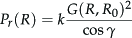
Therefore, the ground model is defined by three features: the intensity k associated with the slant range, the goodness of fit E, and the shape factor S. This set of features is used to model the ground and classify radar returns as ground or non-ground, according to the classification algorithm described in Section 4.2.

5.1.2. Radar: experimental results

Experimental validation of the radar classifier was performed using an off-road vehicle operating in a rural environment. The vehicle was equipped with a 95 GHz frequency modulated continuous wave (FMCW) radar [36] and an approximately co-located camera. During the experiments, the vehicle was remotely driven as the on-board sensors gathered data of the surrounding environment for the successive off-line processing. Typical results obtained from the radar-based classifier are overlaid on the radar and visual image of Figure 2 (ground labels are denoted by green dots, whereas black crosses mark non-ground labels).

For this scene, the distribution of the radar features used in the current ground model is shown in Figure 3. Although, multiple terrain types (sandy+grass) are simultaneously present in the training set, all three histograms exhibit an approximately uni-modal distribution, which can be reasonably modelled with a single multivariate Gaussian.

Figure 3.

Normalized histograms of the radar features for a training set referring to mixed terrain (sand and grass). All the histograms exhibit an approximately uni-modal distribution, which can be reasonably modelled with a single Gaussian.

Figure 4 collects other sample results. Radar-labelled observations are overlaid over the image plane of the camera, which is approximately co-located with the radar (ground labels are denoted by green dots, a black cross marks non-ground). Although, the system is conceived as classifying data that belong to the ground echo, obstacles present in the ‘foreground’ can also be detected and ranged independently as high-intensity peaks [37] (denoted by red triangles). As can be seen from these figures, the classifier correctly detects drivable areas and obstacles present in the scene. Additional results may be found in [29].

Figure 4.

(a) - (b) Radar-based classification results overlaid on the original image for two sample scenes: green dot - classified ground; black cross - classified non-ground; red triangle - foreground obstacle

5.2. Stereo vision classifier

Stereo vision is a common sensing technology used for perception that provides ‘rich’ 3D data (i.e., the raw output from the sensor is a 3D point cloud with associated colour information). Based on geometric features that can be extracted from the stereo vision-generated 3D reconstruction, an adaptive self-taught terrain classifier can be developed [31], [38].

5.2.1. Stereo vision features

The raw 3D point cloud is divided into a grid of o.4 m by 0.4 m terrain patches that are projected onto a horizontal plane. Next, geometric features are extracted from the coordinates of the points that fall in each grid cell. The first element of the geometric feature vector is the average slope of the terrain patch, i.e., the angle θ between the least squares-fit plane and the horizontal plane. The second component is the goodness of fit, E, measured as the mean-squared deviation of the points from the least squares plane along its normal. The third element is the variance in the height of the range data point with respect to the horizontal plane, σ²_h. The fourth component is the mean height of the range data points, h̄.

5.2.2. Stereo vision: experimental results

For the testing and field validation of the stereo vision classifier, a CLAAS AXION tractor was used and operated in a rural environment at a farm near Helsingør, Denmark. It was equipped with a PointGrey Bumblebee XB3 stereo head, as shown in Figure 5. Various scenarios were analysed including positive/negative obstacles, moving obstacles and difficult terrain (slopes, highly-irregular terrain, etc.). Figure 6(a) shows a sample field scenario referring to the bootstrapping process, during which the geometric ground model is initialized at the beginning of the operation. The underlying assumption is that the robot faces relatively even terrain. The output of the stereo vision processing is a 3D point cloud that is first divided into a grid of 0.16 m² cells, as shown in Figure 6(b). Next, feature vectors can be extracted from each cell and the histograms of the distribution of the geometric features are shown in Figure 7. All four histograms exhibit an approximately uni-modal distribution, which suggests that the ground model for this classifier can be reasonably modelled using a single multivariate Gaussian. After the initialization stage, the stereo classifier was able to predict the presence of the ground in successive acquisitions. Some typical results are shown in Figure 8, overlaid on the original image (pixels associated with ground-labelled cells are denoted in green, whereas 3D points falling into cells labelled as non-ground are marked using red dots). As can be seen from these figures, the classifier correctly detects the ground and the obstacles present in the scene [31]. An additional advantage of the proposed approach is that the output traversability map can be directly employed by most grid-based planners [39].

Figure 5.

The tractor test platform employed in this research, along with the description of its sensor suite

Figure 6.

(a) A sample image of a relatively flat area during the bootstrapping process to build the initial model of the ground class. (b) Associated 3D point cloud generated by stereo vision processing and divided into a grid of 0.16 m² cells.

Figure 7.

Normalized histograms of the geometric features for a training window that refers to relatively even agricultural terrain

Figure 8.

(a) - (b) Results obtained from the stereo vision classifier projected over the original camera image for two sample scenes. Pixels associated with ground-labelled cells are marked using green. 3D points associated with non-ground cells are denoted by red dots.

5.3. Radar self-supervised visual classifier

In this section, a novel approach for terrain estimation is presented which combines radar sensing with monocular vision in a self-learning scheme [30]. In detail, the self-taught radar classifier, previously introduced in Section 5.1, is used to find the ground and to supervise the training of a second classifier that uses visual features. In turn, the visual classifier can segment the whole image into ground and non-ground, identifying also those ground regions that are located a significant distance from the camera. In addition, it can further subdivide the ground into subclasses corresponding to different terrain components.

5.3.1. Visual features

Colour and texture cues are adopted to represent ground appearance. Colour data are available as red, green and blue (RGB) intensity components. However, raw RGB space is sensitive to lighting variations and non-uniform illumination conditions. Therefore, it is generally useful to map the colours from the RGB space onto a more suitable one, especially in outdoor contexts [40]. In this implementation, the rg chromaticity space is adopted. The rg chromaticity space contains less information than RGB or HSV colour spaces; however, it has several useful properties for computer vision applications and has been demonstrated to perform similarly to other more complex normalized colour representations (e.g., c1c2c3) [41], [31]. The main advantage of this space is that changes in light intensity do not affect the basic colour of the objects in the scene.

Textural features are useful to represent the local spatial variation in intensity across the image. Several texture descriptors have been proposed in the literature, such as Gabor filters, wavelets and local energy methods [42], [43]. Here, an approach based on the grey level co-occurrence matrix (GLCM) is employed. Haralick et al. [44] have proposed 14 statistical features that can be extracted from a GLCM to estimate the similarity between different GLCMs. Among these features, two of the most relevant are energy and contrast [45]. Energy accounts for the textural uniformity of an image, reaching its highest value when the grey level distribution has either a constant or a periodic form. Contrast measures the amount of local variations in an image. These two parameters have been recognized as being highly significant in discriminating between different textural patterns [46]. Energy and contrast are used in this work to characterize the textural content of the ground.

In summary, two scalar colour descriptors (i.e., the r and g colour components in the chromaticity space) and two scalar textural descriptors (i.e., energy and contrast) are concatenated forming a four-dimensional feature vector. As these features depend upon the visual appearance of the ground, different types of terrain will generate multi-modal histograms, thus requiring a MoG fitting with K > 1, as will be shown later in Section 5.3.3. One should also note that more complex visual descriptors may be employed without changing the rest of the algorithm.

5.3.2. Radar supervision

The radar-based classifier is used to automatically train the vision-based algorithm. With reference to the example of Figure 9, radar-labelled ground observations are first projected over the camera image; then, for each projected point, an attention window is set, as follows. For each ground-labelled radar point, a squared ground patch of 0.30 m × 0.30 m centred on that point is projected over the visual image using the perspective transformation. The resulting bounding box will be a rectangular window (see Figure 9), from which visual features can be extracted to build a training set for the ground class. It should be noted that accurate calibration and synchronization of the sensors needs to be performed to ensure an appropriate re-projection of radar-labelled points on the visual image. Errors in calibration or synchronization may cause incoherency between the data acquired by the two sensors and consequent failure in any stage of the classification system. For instance, points labelled as ‘ground’ by the radar may be wrongly projected onto non-ground regions of the image, thus causing an incorrect training of the visual ground model. For the experimental setup adopted in this work, accurate calibration information is available, including both intrinsic and extrinsic parameters of the camera. Specifically, extrinsic parameters define the relative position of the camera reference frame with respect to the radar reference frame, while intrinsic parameters are used to transform metric point coordinates into pixel coordinates. In addition, the sensors are time-synchronized. The reader is referred to [47] for more detailed information concerning calibration and synchronization.

Figure 9.

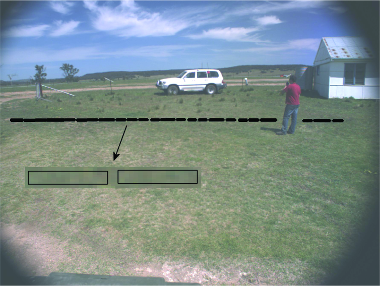
Projections of ground-labelled radar returns over the co-located camera image, along with a close-up of some attention windows. Visual features extracted from these windows are added to the training set to build a visual model of the ground.

The visual algorithm operates on the entire field of view of the camera. A block-based method is used to reduce the segmentation processing time at the cost of a lower resolution. Specifically, the image is divided into small patches and for each sub-image, the feature vector is computed and compared with the current ground model for classification, as explained in Section 4.2.

5.3.3. Radar-supervised visual classifier: experimental results

The system was experimentally validated using the test bed, previously described in Section 5.1.2. A typical result obtained from the radar-supervised classifier is shown in Figure 10, where the terrain mainly consisted of grass and sandy soil. The radar-labelled ground points are projected over the original image and denoted by green crosses, providing training examples to the visual classifier. The number of Gaussian components returned by the EM-BIC algorithm was K = 2. The classification results produced by the visual classifier for the entire video frame are shown in Figure 10(b) and Figure 10(c). Specifically, in Figure 10(b), pixels associated with ground-labelled patches are marked in green, whereas the two terrain subclasses detected by the system are shown as dark green and brown pixels in Figure 10(c). It should be noted that these two colours have been obtained as a result of averaging the RGB colours of the clusterized training samples, thus showing a coherent association between each ground class and its expected colour appearance.

Figure 10.

Field validation: (a) ground-labelled radar points projected over the co-located visual image (green crosses); (b) segmented super-class of the ground (green pixels); (c) identification of two ground subcomponents. In (c), the two terrain types are marked using the average RGB colours of the clusterized training patterns. Note that the blue channel was removed to improve visualization.

In order to underline the merits of the adaptive strategy, a specific data set is considered where the terrain encountered by the vehicle changed from mostly sandy to mostly grass, and to mostly sandy again. Overall, 868 radar images and corresponding visual images were stored. Every tenth image was hand-labelled to build ground truth, resulting in 86 labelled frames. Figure 11 and Figure 12 compare the results obtained from the system both using and not using online ground model updates. Figure 11 shows some salient frames of the sequence, whereas the classification accuracy for each testing image is plotted in Figure 12. In detail, in Figure 11, the first row shows the ground-labelled radar points in the current scan (green crosses) projected over the co-located visual image, whereas in the second and third rows the super-class of the ground is denoted using green coloured pixels, as detected by the visual classifier, using the offline learning approach and the online learning system, respectively. In Figure 12, the accuracy of the online learning algorithm is shown by a solid line with dots, whereas the results for the offline learning approach are denoted by a solid line with crosses. These figures demonstrate that in the first frames (approximately up to the 90 ^th frame) both the online and the offline algorithm performed well, as the ground appearance did not vary significantly. Afterwards, the offline algorithm degraded, until the vehicle returned to its starting position (approximately at frame 800).

Figure 11.

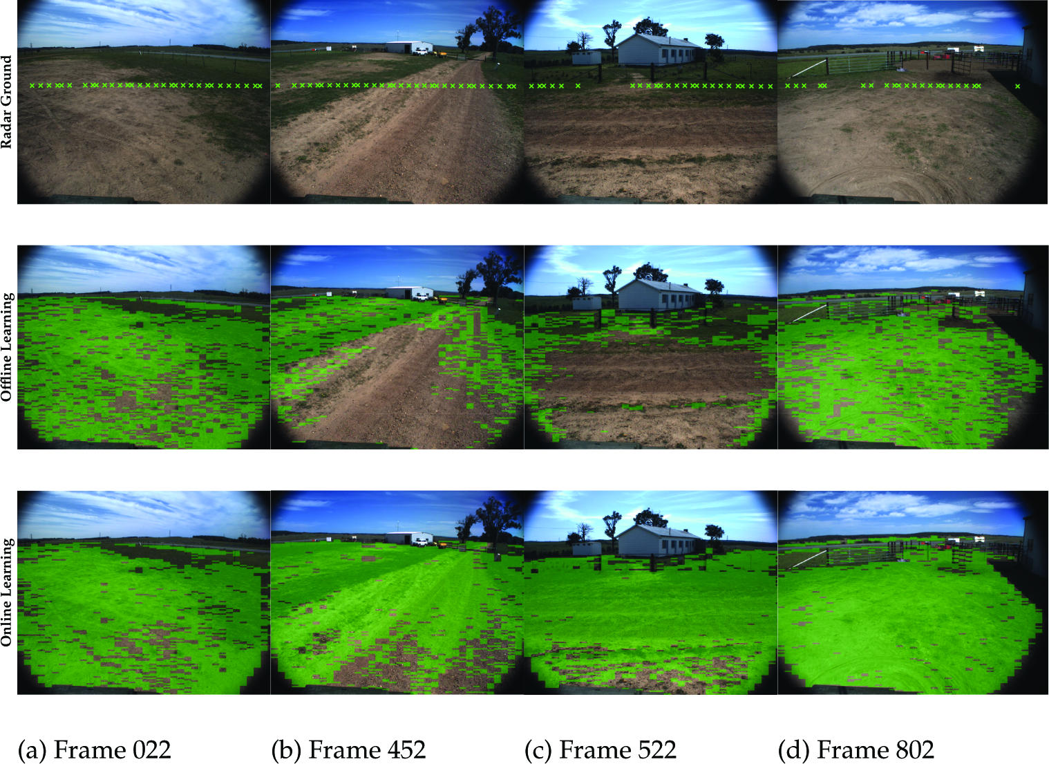
Comparison of the online and offline learning. First row: ground-labelled radar observations (green crosses); second row: output of the offline classifier; third row: output of the online classifier. Note that, in these images, only the super-class of the ground is shown using green pixels.

Figure 12.

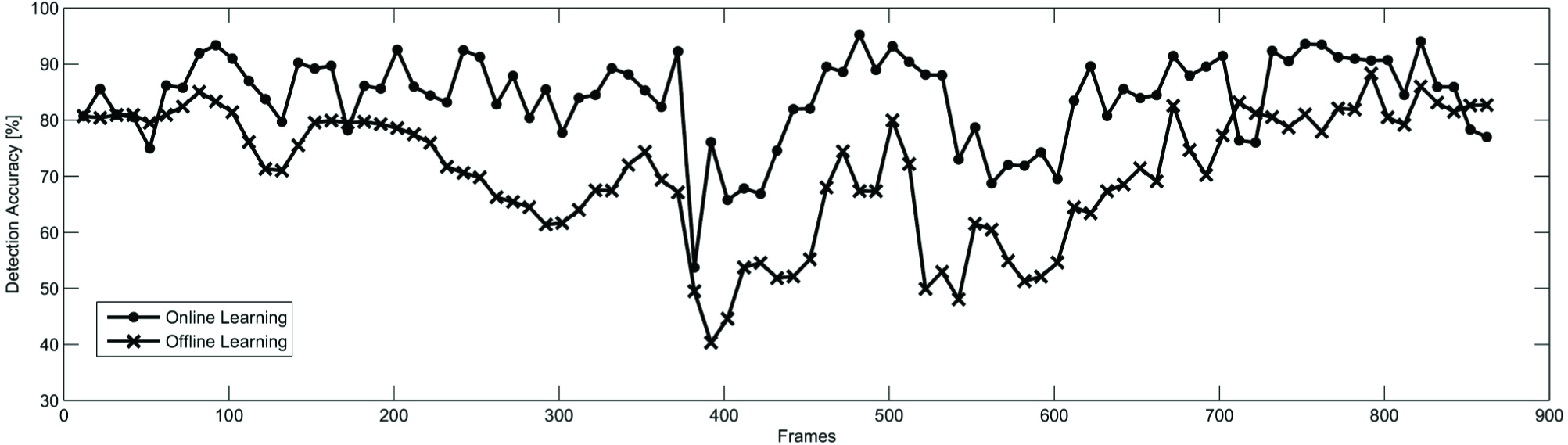
Classification accuracy: solid line with dots - online learning strategy; solid line with crosses - offline learning strategy (i.e., the classifier is trained once at the beginning of the robot operation)

The ability of the online system to recover from poor classification performance can be observed in Figure 13 for frames 382–392, during a left-hand turning manoeuvre performed by the vehicle. Radar-generated training instances of the ground are denoted by green crosses in Figure 13(a)–(b), whereas the results of the visual classification are shown in Figure 13(c)–(d). Initially, only instances of grass were incorporated into the ground model; as a direct consequence, sand was not recognized as ground by the visual classifier (see Figure 13 (a)–(c)) and a corresponding drop in the detection accuracy can be observed in Figure 12. This points to an intrinsic drawback of the online learning approach: a new ground portion will not be recognized as ground until samples of it are added to the ground model. Nevertheless, the online learning algorithm rapidly adapted as soon as instances of sand were added to the training rolling window, such that sand was also segmented as ground (see Figure 13 (b)-(d)), with a consequent increment in the detection accuracy. Table 2 summarizes the classification performance obtained from the system using the online approach as compared to the offline learning system in terms of accuracy and F1-score. Overall, the average accuracy resulted in 70.81% with a standard deviation of 11.34% for the offline learning system, whereas the online learning demonstrated better performance with an average accuracy and standard deviation of 84.07% and 7.80%, respectively.

Table 2.

Radar-supervised visual classifier: accuracy and F1-score using online learning (i.e., with ground model updates) versus offline learning (i.e., without ground model updates)

	Online learning	Offline learning
Mean Accuracy (%)	84.07	70.81
St. Dev. of Accuracy (%)	7.80	11.34

Mean F1-score (%)	85.13	67.71
St. Dev. of F1-score (%)	8.96	16.91

Figure 13.

System adaptation to different terrain types. Initially, the training rolling window includes instances of grass only and sand is not recognized as ground (a)-(c). As soon as enough instances of sand are added, sand is also recognized as ground (b)-(d). In (a) and (b), the green crosses denote ground-labelled radar points. In (c) and (d), image pixels belonging to ground are marked using the average RGB colour of the respective terrain type (the blue channel was removed to improve visualization).

5.4. Stereo-supervised visual classifier

Stereo vision provides ‘rich’ 3D data, including geometric and colour information of the surrounding environment. The two sources of information can be combined into an adaptive self-supervised algorithm for automatic ground detection and characterization [31]. In detail, the classifier - previously described in Section 5.2 - is used to segment the scene into ground and non-ground regions based on geometric data, and labels from this algorithm are used to automatically train a second classifier that performs visual image segmentation.

5.4.1. Colour features

The visual appearance of the ground is represented in terms of colour information. To reduce the effect of the overall illumination level, the RGB information is transformed into the so-called ‘C₁C₂C₃ colour’ model. It should be noted that, since there may be many pixels observed in each terrain patch, the overall estimate of the class likelihood, based on the pixels' colour, is taken as the mean of the class likelihoods of the individual pixels. Thus, the colour properties of each patch are represented as a three-element vector x = [c₁, C₂, C₃]. In the proposed self-supervised framework, colour-feature vectors associated with ground-labelled cells by the stereo-based classifier are automatically used for the colour-based training.

5.4.2. Stereo-supervised visual classifier: experimental results

Experimental validation was performed using the tractor test bed, previously described in Section 5.2.2. Figure 14 shows a sample field scenario where the tractor drives along a dirty road delimited by grassy areas along the side. Colour-feature vectors can be extracted from the training cells provided by the stereo-based classifier. The histograms of their distribution are plotted in Figure 14(c). All three histograms exhibit a multi-modal trend. If EM with BIC is used to fit the MoG a number of components K = 2 is found, as expected given the presence of two main types of terrain in the scene, namely dirty road and grass.

Figure 14.

Results obtained from the stereo-supervised visual classifier as the tractor drives along a dirty road with grass on the side. (a) Original visual image. (b) Segmentation of the entire image. Yellow pixel: dirty road. Green pixel: grass. Red pixel: non-ground. (c) histogram of the distribution of the colour features for the associated training window. The colour-based classifier fits a MoG with K = 2 components, consistent with the presence of dirty road and grass in the scene.

In Figure 14(b), the results obtained from the colour-based classifier are shown. Pixels associated with the first type of terrain (dirty road) are denoted in yellow, whereas pixels corresponding to the second type of ground (grass) are marked using green. Finally, pixels labelled as non-ground are denoted using red.

The system adapts to new terrain by updating the training window online. The sequence in Figure 15 illustrates the adaptation process: Figure 15(a) and Figure 15(c) show the training ground patches as obtained by the stereo-based classifier in two successive frames. Again, points that belong to a cell labelled as ‘ground’ are denoted by green dots, whereas points falling into cells marked as ‘non-ground’ are denoted by red dots. Figure 15(b) and Figure 15(d) display the results of applying the colour-based classifier. As no training instances of grass are initially provided by the stereo-based classifier (Figure 15(a)), grass is not recognized by the system as ground (Figure 15(b)). Nevertheless, as soon as new instances of ground-labelled grass are added to the training rolling window (Figure 15(c)), the algorithm adapts while still correctly labelling obstacles present in the scene (Figure 15(d)).

Figure 15.

A sample sequence showing the rapid adaptation of the system to changes in the appearance of the ground. Figure 15(a) and Figure 15(c) show the results of the geometric classification that supervises the training set of the colour classification shown in Figure 15(b) and Figure 15(d). When the stereo-based classifier predominantly screens the dirty road, grass is not classified as ground. As new instances of grass start populating the rolling training window, the classification changes.

In order to provide a quantitative evaluation of the system performance, the precision and recall of the overall ground classifier were measured for a subset of images (s_b = 40) taken from different data sets. This subset was hand-labelled to identify the ground-truth terrain class corresponding to each pixel. By assuming a typical significance level of 0.05 (α = 95% for the cut-off threshold), it resulted in an average precision of 91.0% and a recall of 77.3%.

6. Conclusions

This paper presented a review of the research carried out by the authors in the context of self-supervised ground detection using different sensor combinations. Specifically, a self-learning framework for online ground detection and characterization in outdoor environments was described. It adopts a MoG to model the ground class and an outlier rejection strategy based on the Mahalanobis distance in order to classify sensory data into ground or non-ground. The system features adaptivity and modularity, as the ground model is learnt and updated in the field during operations. It can easily adjust to changing conditions and environments, which may be useful for long-range navigation in unknown environments. In addition, it can be applied to a single sensor or else to combine multiple sensors according to a self-supervised scheme, thus avoiding time-consuming manual labelling. Two classifiers were presented that identify ground and non-ground regions using radar and stereo data, respectively. They can also serve to automatically train scene classifiers using monocular visual features. All the proposed methods were extensively validated in the field using experimental test beds showing good classification results and demonstrating the ability to adapt to environmental changes, including variations in illumination conditions and ground appearance, after an automatic initialization phase, with no need for manual supervision for training.

Self-learning systems may be a feasible solution when no prior data sets are available for training, and wherever the use of a static ground model would rapidly lead to poor classification results. However, the use of a full self-supervised procedure brings intrinsic limitations. First, sensors need to be accurately calibrated and time-synchronized with respect to each other in order to have a coherent data association, which is a pre-requisite for correct data fusion. Furthermore, the overall accuracy of the classifier depends upon the ability of both the supervising module (to produce a reliable training set) and the robustness of the supervised classifier; therefore, the overall system performance suffers from error propagation. While batch-trained classifiers can take advantage of multiple and simultaneously available training examples, incremental learning systems need to learn sufficient information in order to accommodate new classes that may be introduced with new data before performing accurate scene classification. In the specific case of ground segmentation, portions of ground cannot be properly recognized until they have been included in the training set. This is particularly critical for the radar-vision system adopted in this research, where the supervising sensor (i.e., the radar) has a field of view much narrower than the supervised sensor (i.e., the camera), so that the area where the training samples are collected covers a small portion of the environment, whereas classification is performed on the entire video frame. On the other hand, the system may forget previously acquired knowledge. In the proposed framework, this problem may be partly mitigated by choosing an appropriately sized training rolling window; however, future work by the authors will include research into a strategy to preserve previous knowledge. Future work will also address the specific research on more complex visual features so as to better deal with the underlying structures of the ground and obstacles. Another strand of the research will address the analysis of the system performance given failure conditions for one sensor (e.g., when the radar is affected by specularity and reflection, or when the camera fails due to visual obscurants).

Footnotes

7. Acknowledgements

The financial support of the ERA-NET ICT-AGRI through the grant Ambient Awareness for Autonomous Agricultural Vehicles (QUAD-AV) is gratefully acknowledged. The authors are thankful to the Australian Department of Education, Employment and Workplace Relations for supporting the project through the 2010 Endeavour Research Fellowship 1745_2010. The authors would also like to thank the National Research Council of Italy, for supporting this work under the CNR 2010 Short Term Mobility Programme.

References

Huertas

Matthies

Rankin

. Stereo-based tree traversability analysis for autonomous off-road navigation. In Proceedings of Workshop of Applications of Computer Vision, 2005.

Pagnot

Grandjean

. Fast cross country navigation on fair terrains. In Proceedings of IEEE International Conference on Robotics and Automation, pages 2593–2598, 1995.

Singh

Simmons

Smith

Stentz

Verma

Yahja

Schwehr

. Recent progress in local and global traversability for planetary rovers. In Proceedings of IEEE International Conference on Robotics and Automation, pages 1194–1200, 2000.

DeSouza

Kak

. Vision for mobile robot navigation: A survey. IEEE Transactions on Pattern Analysis and Machine Intelligence, 24(2):237–267, 2002.

Jochem

Pomerleau

Thorpe

. Vision-based neural network road and intersection detection and traversal. In Proceedings of IEEE/RSJ International Conference on Intelligent Robots and Systems, 1995.

Pomerleau

. ALVINN: An autonomous land vehicle in a neural network. In Advances in neural information processing systems: Morgan Kaufmann., 1989.

LeCun

Huang

F. J.

Bottou

. Learning methods for generic object recognition with invariance to pose and lighting. In Proceedings of Conference on Computer Vision and Pattern Recognition, volume 2, pages 97–104, 2004.

Manduchi

Castano

Talukder

Matthies

. Obstacle detection and terrain classification for autonomous off-road navigation. Autonomous Robot, 18:81–102, 2003.

Hong

Chang

Rasmussen

Shneier

. Road detection and tracking for autonomous mobile robots. In Proceedings of SPIE Aerosense Conference, pages 1194–1200, 2002.

10.

Rasmussen

. Combining laser range, color, and texture cues for autonomous road following. In Proceedings of IEEE International Conference on Robotics and Automation, 2002.

11.

Dima

Vandapel

Hebert

. Classifier fusion for outdoor obstacle detection. In Proceedings of International Conference on Robotics and Automation (ICRA), volume 1, pages 665–671, 2004.

12.

Brooks

C.A.

Iagnemma

. Self-supervised terrain classification for planetary surface exploration rovers. Journal of Field Robotics. Special Issue: Special Issue on Space Robotics, Part I, 29 (3):445–468, 2012.

13.

Vernaza

Taskar

Lee

D.D.

. Online, self-supervised terrain classification via discriminatively trained submodular Markov random fields. In Proceedings of IEEE International Conference on Robotics and Automation, pages 2750–2757, 2008.

14.

Dahlkamp

Stavens

Kaehler

Thrun

Bradski

. Self-supervised monocular road detection in desert terrain. In Proceedings of the Robotics Science and Systems Conference, 2006.

15.

Zhou

McDaniel

M.W.

Nishihata

Salesses

Iagnemma

. Self-supervised learning to visually detect terrain surfaces for autonomous robots operating in forested terrain. Journal of Field Robotics, 29(2):277–297, 2012.

16.

Reina

Milella

Halft

Worst

. LIDAR and stereo imagery integration for safe navigation in outdoor settings. In Safety, Security, and Rescue Robotics (SSRR), 2013 IEEE International Symposium on, pages 1–6, 2013.

17.

Peynot

Underwood

Scheding

. Towards reliable perception for unmanned ground vehicles in challenging conditions. In Proceedings of IEEE/RSJ International Conference on Intelligent Robots and Systems, St Louis, MO, USA, 2009.

18.

Reina

Underwood

Brooker

Durrant-Whyte

. Radar-based perception for autonomous outdoor vehicles. Journal of Field Robotics, 28(6):894–913, 2011.

19.

Milella

Reina

Siegwart

. Computer vision methods for improved mobile robot state estimation in challenging terrains. Journal of Multimedia, 1(7):49–61, 2006.

20.

Reina

Ishigami

Nagatani

Yoshida

. Odometry correction using visual slip-angle estimation for planetary exploration rovers. Advanced Robotics, 24(3):359–385, 2010.

21.

Reina

Ishigami

Nagatani

Yoshida

. Vision-based estimation of slip angle for mobile robots and planetary rovers. In IEEE International Conference on Robotics and Automation, pages 486–491, 2008.

22.

Sole

Mano

Stein

G.P.

Kumon

Tamatsu

Shashua

. Solid or not solid: Vision for radar target validation. In Proceedings of IEEE Intelligent Vehicles Symposium, 2004.

23.

Luciw

Weng

Zeng

. Incremental online object learning in a vehicular radar-vision fusion framework. IEEE Transactions on Intelligent Transportation Systems, 12(2):402–411, 2011.

24.

Alessandretti

Broggi

Cerri

. Vehicle and guard rail detection using radar and vision data fusion. IEEE Transactions on Intelligent Transportation Systems, 8(1):95–105, 2007.

25.

Decker

Chang

Camus

Eledath

. Collision sensing by stereo vision and radar sensor fusion. IEEE Transactions On Intelligent Transportation Systems, 10(4):606–614, 2009.

26.

Atreya

Cattle

Momen

Collins

Downey

Franken

Glass

Herbach

Saxe

Ashwash

Baldassano

Javed

Mayer

Benjamin

Gorman

. DARPA Urban Challenge Princeton University. Technical report, 2007.

27.

Milella

Reina

Underwood

Douillard

. Combining radar and vision for self-supervised ground segmentation in outdoor environments. In Proceedings of IEEE/RS] International Conference on Intelligent Robots and Systems (IROS), pages 255–260, 2011.

28.

Milella

Reina

Underwood

Douillard

. Visual ground segmentation by radar supervision. Robotics and Autonomous Systems, 62(5):696–706, 2014.

29.

Reina

Milella

Underwood

. Self-learning classification of radar features for scene understanding. Robotics and Autonomous Systems, 60(11):1377–1388, 2012.

30.

Milella

Reina

Underwood

. A self-learning framework for statistical ground classification using radar and monocular vision. Journal of Field Robotics, Article first published online: 3 APR 2014 DOI: 10.1002/rob.21512.

31.

Reina

Milella

. Towards autonomous agriculture: Automatic ground detection using trinocular stereovision. Sensors, 12(9):12405–12423, 2012.

32.

Zhu

. Semi-supervised learning literature survey. Technical Report 1530, Computer Sciences, University of Wisconsin-Madison, 2005.

33.

Tax

D.M.J.

. One-Class Classification. Concept Learning in the Absence of Counter Examples. PhD thesis, Delft University of Technology, Delft, Netherlands, 2001.

34.

Raftery

A. E.

. Bayesian model selection for social research (with discussion). Sociological Methodology, 25:111–196, 1995.

35.

Mardia

Kent

Bibby

. Multivariate Analysis. Academic Press, London, 1979.

36.

Brooker

Hennessey

Bishop

Lobsey

Durrant-Whyte

Birch

. High-resolution millimeter-wave radar systems for visualization of unstructured outdoor environments. Journal of Field Robotics, 23(10):891–912, 2006.

37.

Reina

Underwood

Brooker

. Short-range radar perception in outdoor environments. In Proceedings of Towards Autonomous Robotics Systems (TAROS), pages 265–276, 2011.

38.

Milella

Reina

. 3D reconstruction and classification of natural environments by an autonomous vehicle using multi-baseline stereo. Intelligent Service Robotics, 7:79–92, 2014.

39.

Rohmer

Reina

Yoshida

. Dynamic simulation-based action planner for a reconfigurable hybrid legwheel planetary exploration rover. Advanced Robotics, 24(8–9):1219–1238, 2010.

40.

Sofman

Lin

Bagnell

J. A.

Vandapel

Stentz

. Improving robot navigation through self-supervised online learning. In Proceedings of Robotics: Science and Systems, 2006.

41.

Gevers

Van De Weijer

Stokman

. Color Feature Detection. Chapter in Color Image Processing: Emerging Applications. CRC Press, 2006.

42.

Reed

Hans du Buf

. A review of recent texture segmentation and feature extraction techniques. Computer Vision, Graphics, and Image Processing, Image Understanding, 57(3):359–372, 1993.

43.

Brooks

C.A.

Iagnemma

. Visual detection of novel terrain via two-class classification. In Proceedings of IEEE/RSJ International Conference on Intelligent Robots and Systems, 2008.

44.

Haralick

R.M.

Shanmugam

Dinstein

. Textural features for image classification. IEEE Transactions on Systems, Man and Cybernetics, 3 (6):21–24, 1973.

45.

Cossu

. Segmentation by means of textural analysis. Pixel, 1 (2):21–24, 1988.

46.

Baraldi

Parmiggiani

. An investigation of the textural characteristics associated with gray level co-occurrence matrix statistical parameters. IEEE Transactions on Geoscience and Remote Sensing, 33 (2):293–304, 1995.

47.

Peynot

Scheding

Terho

. The Marulan Data Sets: Multi-Sensor Perception in Natural Environment with Challenging Conditions. International Journal of Robotics Research, 29(13):1602–1607, November 2010.

Adaptive Multi-Sensor Perception for Driving Automation in Outdoor Contexts

Abstract

Keywords

1. Introduction

2. Literature review

3. Adaptive self-learning

4. Statistical ground classification

4.1. Ground model

4.2. Sensor data labelling

4.3. Model update

5. Automatic ground-detection

5.1. Radar classifier

5.1.1. Radar features

5.1.2. Radar: experimental results

5.2. Stereo vision classifier

5.2.1. Stereo vision features

5.2.2. Stereo vision: experimental results

5.3. Radar self-supervised visual classifier

5.3.1. Visual features

5.3.2. Radar supervision

5.3.3. Radar-supervised visual classifier: experimental results

5.4. Stereo-supervised visual classifier

5.4.1. Colour features

5.4.2. Stereo-supervised visual classifier: experimental results

6. Conclusions

Footnotes

7. Acknowledgements

References