Sage Journals: Discover world-class research

Abstract

For natural human-robot interaction, the location and shape of facial features in a real environment must be identified. One robust method to track facial features is by using a particle filter and the active appearance model. However, the processing speed of this method is too slow for utilization in practice. In order to improve the efficiency of the method, we propose two ideas: (1) changing the number of particles situationally, and (2) switching the prediction model depending upon the degree of the importance of each particle using a combination strategy and a clustering strategy. Experimental results show that the proposed method is about four times faster than the conventional method using a particle filter and the active appearance model, without any loss of performance.

Keywords

Facial Feature Tracking Particle Filter Active Appearance Model Robot Vision Human-robot Interaction

1. Introduction

In order to serve humans efficiently, robots must be able to interact naturally with humans. This requires robots to recognize the emotions, intentions, and states of humans. According to Mehrabian's rule [1], in human-human communication, only seven percent of the information that we send is verbal, 38 percent is sent in acoustic signals, such as tone of voice, and 55 percent is sent through visual signals, such as facial expressions and gestures. Therefore, the ability to understand human non-verbal signals is essential.

The channel for conveying the most information continuously is facial expressions. Tone of voice cannot convey information when humans do not speak. Gestures can be restricted, depending upon human poses and the given situation. However, facial expressions convey information continuously, unless the face is hidden on purpose. Moreover, facial expressions are generally universal and innate, regardless of culture [2, 3]. Therefore, to facilitate natural human-robot interaction, facial expression recognition systems must be prioritized. Facial expression recognition systems are implemented in four steps: 1) face detection, 2) facial feature extraction, 3) facial-action detection, and 4) emotion, intention and state recognition. The performance of steps 3) and 4) depends upon the performance of steps 1) and 2). In the current systems, step 1) works well to some degree. However, step 2) remains a challenging problem.

The face conveys information using the movement of numerous muscles. This movement is mostly expressed by the eyebrows, eyes, nose and mouth. Therefore, the features to be extracted from a facial image are the location and shape of the eyebrows, eyes, nose and mouth.

The most representative method for extracting facial features is the Active Appearance Model (AAM) [4]. This method is widely used for facial expression recognition [5], facial image analysis [6], face recognition [7], eye modelling [8] and medical image analysis [9]. However, due to the nature of the algorithm, the AAM is sensitive to initial conditions and environmental changes. For this reason, the AAM has some difficulties concerning its application in real service situations.

Many methods to strengthen the ability of the AAM have been proposed. In [10], an analytic fitting method based on an inverse compositional image alignment algorithm has been proposed. In [11], Canonical Correlation Analysis (CCA) has been applied to the AAM for fast searching. In [12], Bayesian Tensor Analysis (BTA) has been applied to the AAM to model 3D faces. In [13], a 2.5D AAM has been proposed, which can outperform the 2D + 3D combined approach as well as the 2D approach. In [14], bidirectional warping has been proposed, which warps both the input image by the affine transform and the template by the inverse compositional image alignment algorithm. In [15], the Hough voting-based method using kernel density estimation has been proposed, which constructs and uses a local voting map to effectively constrain the search region. The above methods mostly deal with one-shot image analysis. However, in real service situations, a robot is input an image sequence consistently. Hence, any such robot should deal with an image sequence. However, an increase in the number of images means not only an increase in amount of the information but also an increase in the level of noise. In addition, the efficiency of a method must be considered. We will look at this problem from the perspective of tracking.

When the AAM is applied to tracking, it is generally used by searching each subsequent frame that employs the result of the previous frame for initialization. However, this approach sometimes fails when somewhat large variations between two frames appear.

There have been successful tracking methods using the AAM. In [16], the cylinder head model has been utilized, in [17] a view-based AAM has been utilized, and in [18] a view-based Active Shape Model (ASM) has been utilized. However, although these methods have focused on pose variation they neglect many variations, such as light variation, background variation, motion blurring, facial expression variation, and occlusion. In addition, some robust methods used a special sensor rather than a typical camera. A 3D TOF camera was used in [19] and a structured light sensor was used in [20].

Recently, more robust, accurate and generally applicable methods have been proposed. A shape prior model based on Restricted Boltzmann Machines (RBMs) was proposed to capture face shape variations in [21]. A regression-based method for automatic AAM initialization during tracking was proposed in [22]. However, these methods do not consider computational efficiency. Consequently, these cannot be applied in real service situations.

One of the robust methods for facial feature tracking uses a particle filter [23, 24], which is widely used for object tracking and robot localization. Handling large numbers of hypotheses, this method can reduce performance variation by setting an initial condition, and it can be robust to environmental changes. However, it has the disadvantage of increasing the computational cost. Previous research [25 –27] has attempted to reduce the state space to solve this problem. However, these approaches are difficult to use in understanding emotions, intentions and states because these methods can only approximate the location and shape of facial features. In other words, they provide insufficient information for understanding emotions, intentions and the states of humans.

In this paper, we propose two ideas to reduce the computational cost of the method using a particle filter without affecting performance.

This paper is organized as follows. In Section 2, the AAM is briefly explained. In Section 3, the conventional particle filter is briefly explained. Section 4 describes the proposed ideas. Section 5 shows the performance of the proposed ideas. Finally, conclusions are provided.

2. Active Appearance Model

The AAM is a powerful method for modelling deformable objects that has been very popular in recent years due to its excellent performance.

2.1. Modelling

The AAM consists of a shape model and a texture model. The shape is the location of the feature points. If there are h feature points, the shape vector can be represented as (1). The texture is the pixel intensities or colors. If the image consists of f pixels, the texture vector can be represented as (2):

s = (x_{1}, ..., x_{h}, y_{1}, ..., y_{h})^{T}

(1)

t = (r_{1}, g_{1}, b_{1}, ..., r_{f}, g_{f}, b_{f})^{T}

(2)

The shape vectors are aligned by Procrustes analysis [28]. Next, the shape model is obtained by applying Principal Component Analysis (PCA) [29] to the aligned shape vectors. The shape model can be represented as (3):

s = \bar{s} + P_{s} b_{s}

(3)

where s̄ is the mean shape vector, P_s is the matrix of the basis vectors of the shape model, and b_s is the shape parameter.

Each training image is warped into the mean shape. As a result, we obtain shape-free images from which the texture vectors are created by extracting the pixel intensities. The normalized texture vectors are obtained by (4). The texture model is then obtained by applying PCA to the normalized texture vectors. The texture model can be represented as (5):

t = (t_{i m} - β 1) ∕ α

(4)

t = \bar{t} + P_{t} b_{t}

(5)

where t_im is the texture vector before normalization, 1 is the vector of 1s, α and β are the standard deviation and mean of the elements of the texture vector, respectively, t̄ is the mean texture vector, P _t is the matrix of the basis vectors of the texture model, and b _t is the texture parameter.

In order to obtain the final AAM, PCA is applied once more to the concatenated shape and texture parameters. The final AAM can be represented as (6):

b = P_{c} c

(6)

where P _c is the matrix of the basis vectors of the AAM, and c is the AAM parameter that can control both the shape model and the texture model.

The number of the basis vectors is chosen so that the model preserves some proportion of the total variance in the training set. Since each eigenvalue reflects the variance of the direction of the corresponding eigenvector, we can choose the number of the basis vectors as the smallest τ satisfying (7):

\sum_{i = 1}^{τ} λ_{i} \geq ξ \times \sum_{i = 1}^{a} λ_{i}

(7)

where λ_i is the i-th eigenvalue, a is the number of eigenvalues, τ is the number of basis vectors of the model, and ξ is the proportion of the total variance to preserve. In this paper, we use 0.98 as the value of ξ.

2.2. Fitting

The objective of fitting is to minimize the difference between the input image and the generated image from the model by adjusting the model parameters. The cost function can be represented as (8):

r (p) = t_{s} - t_{m}

(8)

where p^T = (c^T|q^T), q is the pose parameter consisting of the scale parameter, rotation parameter and location parameter, t_s is the texture vector from the input image, and t_m is a texture vector generated from the model.

The AAM assumes that there is a linear relationship between the variance of the model parameter δp and the residual r(p), which can be represented as (9):

δ p = R r (p)

(9)

where R is the linear relationship between δp and r(p).

The AAM also assumes that R is fixed and pre-computes it by using training data. Specifically, the fitting procedure is performed by iteratively updating the parameter using (9) until there is no more improvement.

3. Particle Filter

The particle filter is an estimation technique based on simulation, which is also known as the ‘sequential Monte Carlo method’. The particle filter is an implementation of a recursive Bayes filter using importance sampling. The key idea of the particle filter is to represent the posterior probability distribution by a set of randomly chosen weighted samples that are called ‘particles’. As the number of particles approaches infinity, the characterization becomes an equivalent representation of the true posterior probability distribution. Due to its flexibility in application to nonlinear and non-Gaussian systems, the particle filter is widely used for visual object tracking and robot localization.

The set of particles can be represented as (10):

S_{t} = {​ < x_{t}^{(i)}, w_{t}^{(i)} > ​ | ​ ​ i = 1, 2, ..., n ​}

(10)

where x_t⁽ⁱ⁾ is the state of the i-th particle at time t, and w_t⁽ⁱ⁾ is the weight of the i-th particle at time t.

The particle filter process is divided into three steps: prediction, observation, and re-sampling.

The first step is the prediction step. Using a set of particles at a previous time (t-1) and the prediction model, it estimates a set of particles at the current time (t). The prediction step can be represented as (11):

p (x_{t} | z_{1 : t - 1}) = \int p (x_{t} | x_{t - 1}) p (x_{t - 1} | z_{1 : t - 1}) d x_{t - 1}

(11)

where x_t is the state at time t, z₁:t–1 is the set of observations from time 1 to time t-1, and p(x_t|x_t–1) is the prediction model (also called the ‘process model’).

The second step is the observation step. Using the observed information and the observation model, it weights each particle. This is to correct the result predicted in the prediction step. The ‘weight’ means the likelihood that a particle is in a good state. The observation step can be represented as (12):

p (x_{t} | z_{1 : t}) = \frac{p (z_{t} | x_{t}) p (x_{t} | z_{1 : t - 1})}{p (z_{t} | z_{1 : t - 1})}

(12)

where p(z_t|x_t) is the observation model.

The third step is the re-sampling step, which draws particles in proportion to their weight with replacement. The re-sampling step can be interpreted as a probabilistic implementation of the Darwinian idea of survival of the fittest. After a few iterations without a re-sampling step, most particles have negligible weights. This problem is called the ‘degeneracy problem’. In order to solve this problem, the re-sampling step is required.

At each time, the particle filter repeats the steps above.

4. Facial Feature Tracking Using an Efficient Particle Filter and the Active Appearance Model

The AAM is a suitable method for tracking facial features. However, it has a problem in that it is sensitive to the initial conditions and environmental changes. When trying to solve these problems using a particle filter, another problem that results in a decrease in the processing speed.

In this paper, we propose ideas to increase the processing speed without affecting the performance.

Figure 1 shows an overview of the proposed system. The input is the image sequence at the top and the output is the estimated facial feature vectors at the bottom.

Figure 1.

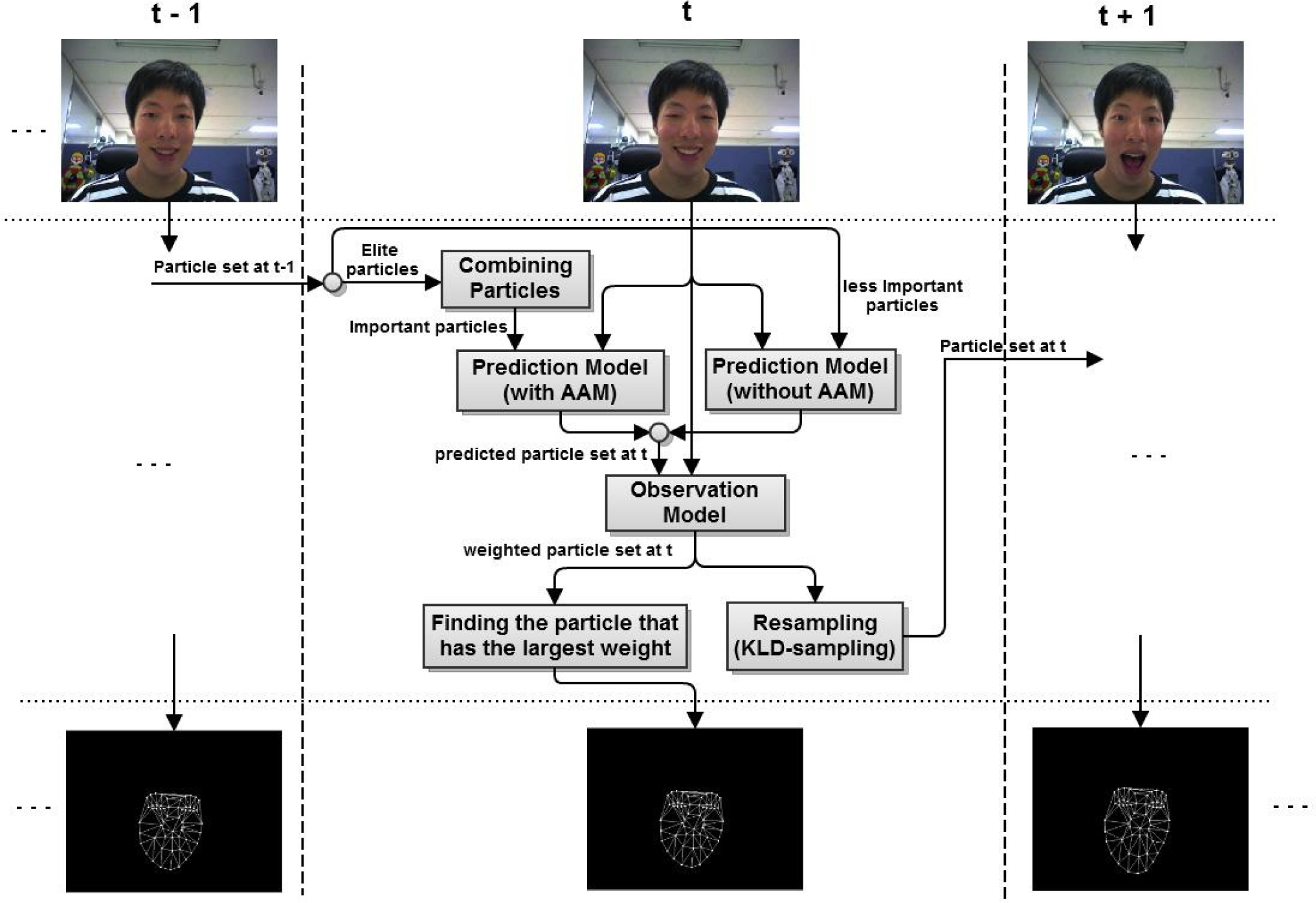
A conceptual diagram of the facial feature tracking method using an efficient particle filter and the active appearance model

First of all, the facial feature vector must be defined. The facial feature vector must deal with both the local motion of the face as well as its global motion. Therefore, the facial feature vector is defined as a vector concatenating pose parameter and a AAM parameter. The pose parameter represents the global motion – position, scale, and rotation – of the face. The AAM parameter represents the local motion and texture of the face. At time t, the facial feature vector can be expressed as (13):

x_{t} = [c_{t}, q_{t}]

(13)

where c_t is the AAM parameter and q _t is the pose parameter.

The information sending from the previous time to the current time is a set of particles, which means the distribution of the facial feature vectors suited to the previous time. The information from the previous time and the current time image are input to the prediction model. The prediction model predicts the distribution of the facial feature vectors suited to the current time. In this paper, we use two different prediction models. For important particles that are acquired by a combination strategy, a prediction model with the AAM is used. For less important particles, a prediction model without the AAM is used. We will look at this in detail in Section 4.1.

The result of the prediction model and the current time image are input into the observation model. The output of the observation model is a set of weighted particles. Namely, the observation model corrects the set of particles predicted by the prediction model.

The observation model is defined as (14):

w_{t}^{(i)} = e x p (- | r (x_{t}^{(i)} {) |}^{2})

(14)

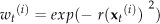
where r(·) is the residual vector defined as (8), which is the difference between the generated image from the AAM and the input image.

If the residual of a particle is low, the observation model judges that this particle is a good state candidate and gives a high weight to this particle. After weighting all the particles, the weights should be normalized so that the sum of the normalized weights is 1.

The next step is to find a particle that has the largest weight. The facial feature vector of this particle is the estimate that is suitable for the current time.

Finally, the particles are re-sampled in proportion to their weights and transmitted to the next time. At that time, we re-sample the least number of particles, as needed. We will discuss this in detail in Section 4.3.

At each time, the proposed system performs the steps above.

In the following subsections, we will discuss in detail the methods that increase the processing speed.

4.1. Efficient prediction step using two prediction models and a combination strategy

The prediction model using the AAM can be defined as (15):

x_{t}^{(i)} = x_{t - 1}^{(i)} + Δ_{t}^{(i)} + S u

(15)

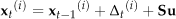
where δ _t ⁽ⁱ⁾ is the predicted amount of change in the parameter. This is an output of the AAM algorithm when the image of the current time (t) and the estimated parameter at the previous time (t-1) are input as the initial conditions. S is the noise covariance matrix, which sets the range of the noise. This allows for uncertainty of estimation. Based on the eigenvalue corresponding to each basis of the AAM, the range can be set because the eigenvalue means the variance of the corresponding basis. u is the Gaussian random number that obeys the normal distribution.

The performance of the prediction model using the AAM is good. However, its computational complexity is too large to be applied for all particles. In the method using the particle filter and the AAM, part of the prediction model accounts for many portions of computational complexity over the entire algorithm because the prediction model includes the output of the AAM as the number of particles. Accordingly, in this paper, in order to reduce the computational complexity effectively, we propose applying a light prediction model for relatively less important particles.

In other words, the prediction model with the AAM as (15) is applied for particles with high weights, and the prediction model without the AAM as (16) is applied for particles with low weights. The prediction model without the AAM is a simple model that adds random noise to the previous state.

x_{t}^{(i)} = x_{t - 1}^{(i)} + S u

(16)

For more effective processing, we employ a combination strategy based on the combining decision rule that generates new rules by creating numerically weighted combinations of existing rules. It is proved for the decision rules generated from a combination strategy to produce better outcomes than different rules that are selected probabilistically [30]. We select the elite particles and combine all pairs of these elite particles as (17). Next, the selected elite particles and the combined elite particles are input to the prediction model with AAM.

x = \frac{w_{1} x_{1} + w_{2} x_{2}}{w_{1} + w_{2}}

(17)

where w is the weight of the particle.

The performance of the AAM is sensitive to the initial condition. That is, when the initial condition is poor, the probability that the prediction model with the AAM does not work properly is high. Therefore, even if the prediction model with the AAM is not applied for particles with low weights, the performance of the entire algorithm is not influenced. In some cases, it prevents the divergence of the particles such that performance can be increased.

4.2. Selection of elite particles

As mentioned earlier, we use two different prediction models to increase the processing speed. In order to do this, we must divide the particles into two groups: elite and non-elite. How do we select the elite particles (or how do we discriminate between the particles)? We propose two methods for selecting the elite particles, and the experimental results are shown in Section 5.

The first method uses the importance of effective samples. We can calculate the effective sample size (ESS) [31] by the variance of particles with respect to their weights as (18). We then define the total importance of the effective samples as the sum of the weights of the effective samples.

E S S = \frac{1}{\sum_{i = 1}^{N} {(w_{i})}^{2}}, ​ ​ w h e r e \sum_{i = 1}^{N} w_{i} = 1

(18)

We assume that elite particles occupy most of the total importance, so we can divide the particles into two groups by using the preservation ratio of the importance of the effective samples. First, the particles are sorted in descending order with respect to their weights. Next, we divide them using the minimum number (N) that satisfies (19):

\sum_{i = 1}^{N} w_{i} ​ \geq ​ η \times \sum_{i = 1}^{E S S} w_{i}

(19)

where η is the preservation ratio. The range of the preservation ratio is from 0 to 1.

This method needs a parameter called the ‘preservation ratio’, which determines the ratio of the elite particles' importance to the total importance. When a parameter is well tuned, the proposed system performs best. However, we cannot guarantee finding the optimal parameter suited to every situation. The experimental results illustrating this are given in Section 5. For this reason, it is difficult to apply this method to real environments.

The second method that supplements the weakness of the first method is the use of k-means clustering [32]. K-means clustering is a simple and useful clustering algorithm. It does not require any parameters except k, which denotes the number of clusters. In our case, since the particles can be divided into important particles and less important particles, k is naturally chosen as 2.

We perform k-means clustering in the weight space so that the particles are divided into two groups. We then choose the group that has higher importance than the other group as the elite particles. Namely, we can select the elite particles without any parameters using this method. Thus, we anticipate that this method would works well in real environments.

4.3. Adaptive number of particles for an efficient particle filter

The computational cost of the particle filter is proportional to the number of particles. Accordingly, if each frame uses a suitable number of particles, it will be possible to reduce the computational cost effectively without affecting the performance. In this paper, we propose a method that situationally adjusts the number of particles using KLD-sampling [33].

KLD-sampling computes the suitable number of particles at each time step using Kullback-Leibler divergence (KL divergence). KL divergence measures the difference between two probability distributions. The difference between the probability distributions p and q can be represented as (20):

K (p, q) = \sum_{x} p (x) l o g \frac{p (x)}{q (x)}

(20)

The objective of the particle filter is to estimate the posterior probability distribution using a set of particles. Specifically, we have to find the least number of particles that maintain the difference between the true posterior probability distribution and the probability distribution estimated by the set of particles. It can be represented as (21):

P (K (\hat{p}, p) \leq ϵ) = 1 - δ

(21)

where p is the true posterior probability distribution, p̂ is the probability distribution estimated by a set of particles, ε is the maximum permissible error between p and p̂, and 1 − δ is the probability that the difference between p and p̂ is less than ε.

The multiplication of the KL divergence and the number of samples n can be represented as the likelihood ratio λ _n , as shown in (22):

l o g λ_{n} = n K (\hat{p}, p)

(22)

The double likelihood ratio can be approximated to the chi-square distribution with k-1 degrees of freedom [34]. It can be applied to (21) as (23):

\begin{array}{l} P (K (\hat{p}, p) \leq ϵ) = P (2 n K (\hat{p}, p) \leq 2 n ϵ) \\ = P (2 l o g λ_{n} \leq 2 n ϵ) \\ \approx P (χ^{2}_{k - 1} \leq 2 n ϵ) \end{array}

(23)

To satisfy (21) and (23), 2nε is equal to X²k−1,1−δ· X²k−1,1−δ is the quantile, which is the output of the inverse function of the cumulative distribution function of the chi-square distribution input 1 − δ. Finally, the least number of particles n is as (24):

n = \frac{1}{2 ϵ} χ^{2}_{k - 1, 1 - δ}

(24)

Approximating the quantiles of the chi-square distribution by Wilson-Hilferty transformation [35], the least number of particles n is as (25):

n \approx \frac{k - 1}{2 ϵ} {1 - \frac{2}{9 (k - 1)} + \sqrt{\frac{2}{9 (k - 1)} z_{1 - δ}}}^{3}

(25)

where z₁−δ is the quantile of the standard normal distribution, which can be readily found from the standard normal distribution chart.

From this result, although we do not know the true posterior probability distribution, the suitable number of particles can be found using the function of the degrees of freedom k-1. According to [33], k can be defined as the number of non-empty bins.

During the re-sampling step, every time a particle is sampled, the algorithm compares the required number of particles with the number of sampled particles. If the number of sampled particles is less than the required number of particles, the re-sampling step is performed once more. Otherwise, the re-sampling step is stopped. At an early stage, the required number of particles and the number of sampled particles increase concurrently. However, over time, the number of non-empty bins k increases only occasionally. Next, the number of sampled particles will finally reach the required number of particles and the re-sampling step will be stopped.

5. Experimental Results

5.1. Experimental environment

The training set used for building a facial AAM model consists of 30 images that have the facial expression variations and pose variations of one person. Each image of the training set is manually annotated at 58 feature points. Some images of the training set are represented as shown in Figure 2. The test sets are the image sequences that are captured in three different environments. The person of the test sets is the same person as the training set. This is because we do not seek to focus on developing and testing a generic facial model but rather on developing and testing the robustness of the method to environmental variations. The ground truth facial feature vectors of the test sets are manually annotated at 58 points in the same way as the training set. Some images of the test sets are represented in Figure 3, Figure 4, and Figure 5. The first test set involves extreme facial expression variation and pose variation. Moreover, lighting variation and blurring also occur due to the pose variation. The first test set contains 104 images. The second test set is a walking situation in a corridor. The background and lighting conditions are continuously varied, and there is also blurring. The second test set contains 174 images. The third test set is a talking situation that involves pose, facial expression, and lighting variations with a complex background. The third test set contains 140 images. The resolution of all the images is 320×240. The training set and the test sets that were used in this paper are available at http://incorl.hanyang.ac.kr/xe/?mid=facedata

Figure 2.

Some images of the training set used for modelling the facial AAM

Figure 3.

Some images of test set #1. It contains extreme facial expression variation and pose variation

Figure 4.

Some images of test set #2. It is a walking situation in the corridor. It contains background variation, lighting variation, and blurring

Figure 5.

Some images of test set #3. It is a talking situation with a complex background. It contains facial expression variation, pose variation, and lighting variation

The specifications of the PC used for the experiments are: Intel i7 3.4 GHz CPU and 16 GB RAM. The implementation of the algorithm was done using C++ and OpenCV 2.0.

5.2. Tracking performance when using the conventional particle filter

First, the tracking performance when using the conventional particle filter is shown by comparing it with the method using the AAM only.

There are two types of experimental schemes for the method using the AAM only. One is a frame-by-frame scheme that initializes each frame afresh. The other is an image sequence scheme that initializes with the previous frame's result. We use a conventional particle filter with the number of particles fixed.

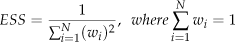
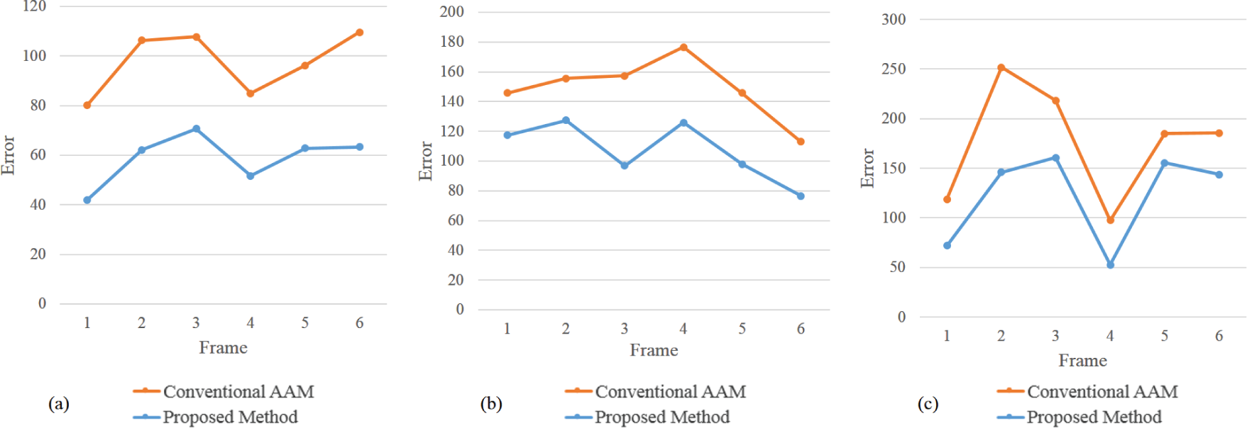
Figure 6 shows the results graphs and compares the three methods. Here, ‘error’ is defined as (26):

Figure 6.

Graphs that show the effect of using a particle filter: (a) result of test set #1, (b) result of test set #2, (c) result of test set #3

e (\hat{x}, x) = \sqrt{\sum_{i} {({\hat{x}}_{i} - x_{i})}^{2}}

(26)

where ◯ is the facial feature vector from the algorithm and x is the ground truth facial feature vector.

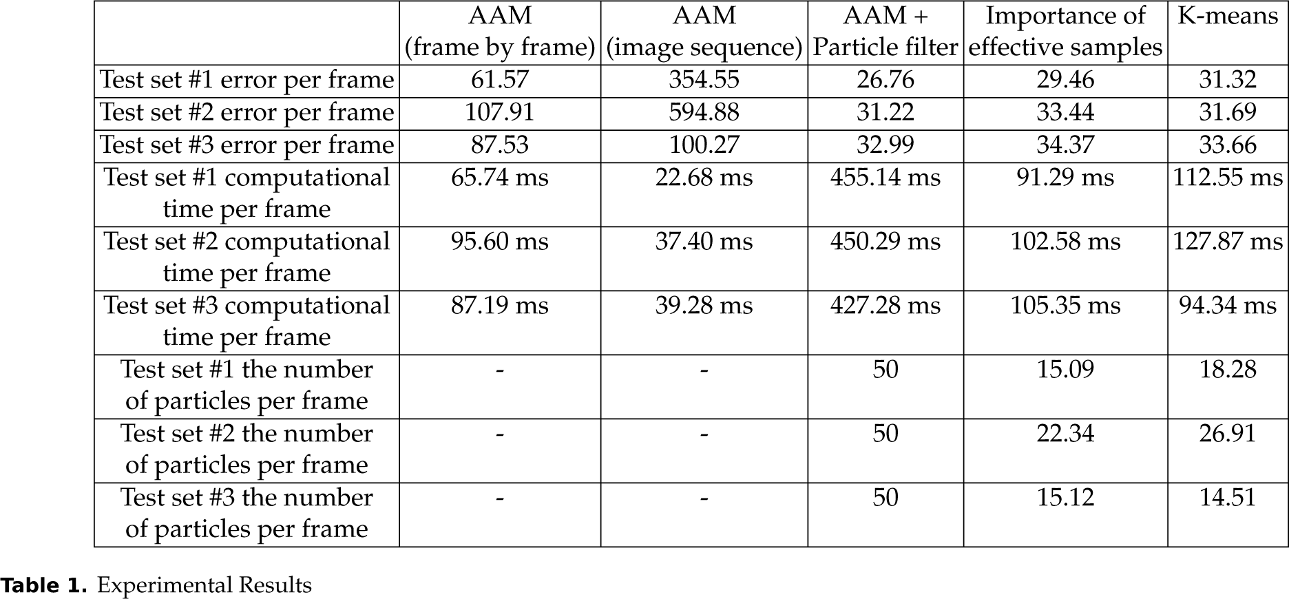
As we can easily see, the performance of the method using a particle filter is more accurate and stable than the method using the AAM only. Refer to Table 1 for details. The second column of Table 1 shows the experimental results of the method using the frame-by-frame scheme of the AAM; the third column of Table 1 shows the experimental results of the method using the image sequence scheme of the AAM; and the fourth column of Table 1 shows the experimental results of the method combining the conventional particle filter and the AAM. We can see that the errors of all the test sets using the conventional particle filter are lower than both the errors of all the test sets using the AAM only.

Table 1.

Experimental Results

	AAM (frame by frame)	AAM (image sequence)	AAM + Particle filter	Importance of effective samples	K-means
Test set #1 error per frame	61.57	354.55	26.76	29.46	31.32
Test set #2 error per frame	107.91	594.88	31.22	33.44	31.69
Test set #3 error per frame	87.53	100.27	32.99	34.37	33.66
Test set #1 computational time per frame	65.74 ms	22.68 ms	455.14 ms	91.29 ms	112.55 ms
Test set #2 computational time per frame	95.60 ms	37.40 ms	450.29 ms	102.58 ms	127.87 ms
Test set #3 computational time per frame	87.19 ms	39.28 ms	427.28 ms	105.35 ms	94.34 ms
Test set #1 the number of particles per frame	–	–	50	15.09	18.28
Test set #2 the number of particles per frame	–	–	50	22.34	26.91
Test set #3 the number of particles per frame	–	–	50	15.12	14.51

5.3. Tracking performance when using the proposed method

In order to know the tracking performance when using the proposed method, we compare it with the method using the conventional particle filter of which the experimental results are represented in the fourth column of Table 1. The fifth column of Table 1 shows the experimental results of the method using the adaptive number of particles and the importance of the effective samples. The last column of Table 1 shows the experimental results of the method using the adaptive number of particles and k-means clustering. Although the mean error per frame for these methods is slightly larger than that is the case using the conventional particle filter method, there is no significant difference. However, its computational speed is about four times faster than for the conventional particle filter method.

Figure 7 shows the number of particles used at each frame. We can see that the range of the number of particles is wide. This means that the number of required particles at each frame varies. Therefore, it is clear that using an adaptive number of particles improves the efficiency of the facial feature tracking system.

Figure 7.

Graphs of the number of particles used at each frame: (a) result of test set #1, (b) result of test set #2, (c) result of test set #3

The results of test set #1 and test set #2 show that the method using the importance of the effective samples has the best results when the parameter is well tuned. However, in the general case, and as we can see from the results of test set #3, it is expected that the method using k-means clustering has the best results. Therefore, we can conclude that using k-means clustering for selecting the elite particles is reasonable.

5.4. Tracking performance under partial occlusion

In order to investigate robustness to partial occlusion, a test set under partial occlusion was created by generating synthetic occlusions onto test set #1. There are three occlusion sequences. The length of each sequence is six frames. The first occlusion sequence is generated around the mouth. An image of the first occlusion sequence is shown in the first column of Figure 8. The second occlusion sequence is generated around the left eye. An image of the second occlusion sequence is shown in the second column of Figure 8. The third occlusion sequence is generated around the right eye. An image of the third occlusion sequence is shown in the third column of Figure 8.

Figure 8.

Images to show the tracking performance under partial occlusion. The images in the first row are test images under partial occlusion, the images in the second row are result images using the AAM only, and the images in the third row are result images using the proposed method.

The result images using the AAM only are shown in the second row of Figure 8, and the result images using the proposed method are shown in the third row of Figure 8. We can see that the facial mesh of the proposed method is well fitted compared to the facial mesh using the AAM only.

To clarify, the experimental results are represented in graph form. Figure 9 (a) represents the experimental results in the case of mouth occlusion, Figure 9 (b) represents the experimental results in the case of left eye occlusion, and Figure 9 (c) represents the experimental results in the case of right eye occlusion. We can see that the error of the proposed method is lower than the error of the AAM only in all frames.

Figure 9.

Graphs that represent tracking performance under partial occlusion: (a) a graph of experimental results for mouth occlusion images, (b) a graph of experimental results for left eye occlusion images, and (c) a graph of experimental results for right eye occlusion images

In fact, the basic AAM is inherently sensitive to occlusion because it models the entire face. However, the proposed method which includes the basic AAM can deal with temporally partial occlusion to some degree because it chooses the best from among the hypotheses that are represented by the particle set.

6. Conclusion and Future Work

In this paper, in order to improve the efficiency of the method using the AAM and the particle filter for robustly tracking facial features under various conditions, we proposed two ideas. The first is to use an adaptive number of particles, which selects a suitable number of particles situationally. The second is to use two different prediction models with a combination strategy, which combines the elite particles and applies the prediction model with the AAM to the combined elite particles. For the other particles, the prediction model without the AAM is applied.

By comparing the proposed method with the method using the conventional particle filter, both ideas improve the processing speed without affecting performance. Consequently, the proposed method is about four times faster than the method using the conventional particle filter.

In the future, we will optimize the code of the proposed method to further improve its speed and extend it to facial expression recognition systems for natural human-robot interaction.

Footnotes

7. Acknowledgements

This work was supported by the Industrial Strategic Technology Development Program (10044009) funded by the Ministry of Trade, Industry and Energy (MOTIE, Republic of Korea).

References

Mehrabian

Albert

. Communication without words. Psychological Today, 2:53–55, 1968.

Ekman

Paul

and Oster

Harriet

. Facial expressions of emotion. Annual review of psychology, 30(1):527–554, 1979.

Irenaus Eibl-Eibesfeldt. The expressive behavior of the deaf-and-blind-born. Social communication and movement, pages 163–194, 1973.

Cootes

Timothy F.

Edwards

Gareth J.

, and Taylor

Christopher J.

Active appearance models. Pattern Analysis and Machine Intelligence, IEEE Transactions on, 23(6):681–685, 2001.

Tao

Dacheng

Song

Mingli

Xuelong

Shen

Jialie

Sun

Jimeng

Xindong

Faloutsos

Christos

, and Maybank

Stephen J

. Bayesian tensor approach for 3-d face modeling. Circuits and Systems for Video Technology, IEEE Transactions on, 18(10):1397–1410, 2008.

Edwards

Gareth J

Taylor

Christopher J

, and Cootes

Timothy F

. Interpreting face images using active appearance models. In Automatic Face and Gesture Recognition, 1998. Proceedings. Third IEEE International Conference on, pages 300–305. IEEE, 1998.

Edwards

Gareth

Cootes

Timothy

, and Taylor

Christopher

. Face recognition using active appearance models. Computer Vision–ECCV'98, pages 581–595, 1998.

Wan

Jian

and Ren

XuePing

. Automatic red-eyes detection based on aam. In Systems, Man and Cybernetics, 2004 IEEE International Conference on, volume 7, pages 6337–6341. IEEE, 2004.

Mitchell

Steven C.

Lelieveldt

Boudewijn P. F.

Van Der Geest

Rob J

Bosch

Hans G

Reiver

JHC

, and Sonka

Milan

. Multistage hybrid active appearance model matching: Segmentation of left and right ventricles in cardiac mr images. Medical Imaging, IEEE Transactions on, 20(5):415–423, 2001.

10.

Matthews

and Baker

Active appearance models revisited. International Journal of Computer Vision, 60(2):135–164, 2004.

11.

Donner

Reiter

Langs

Peloschek

, and Bischof

Fast active appearance model search using canonical correlation analysis. Ieee Transactions on Pattern Analysis and Machine Intelligence, 28(10):1690–1694, 2006. Donner, Rene Reiter, Michael Langs, Georg Peloschek, Philipp Bischof, Horst.

12.

Tao

Dacheng

Song

Mingli

Xuelong

Shen

Jialie

Sun

Jimeng

Xindong

Faloutsos

Christos

, and Maybank

Stephen J.

Bayesian tensor approach for 3-d face modeling. Ieee Transactions on Circuits and Systems for Video Technology, 18(10):1397–1410, 2008.

13.

Martins

Pedro

Caseiro

Rui

, and Batista

Jorge

. Generative face alignment through 2.5d active appearance models. Computer Vision and Image Understanding, 117(3):250–268, 2013.

14.

Mollahosseini

and Mahoor

M.H.

Bidirectional warping of active appearance model. In Computer Vision and Pattern Recognition Workshops (CVPRW), 2013 IEEE Conference on, pages 875–880, June 2013.

15.

Jin

Xin

Tan

Xiaoyang

, and Zhou

Liang

. Face alignment using local hough voting. In Automatic Face and Gesture Recognition (FG), 2013 10th IEEE International Conference and Workshops on, pages 1–8, April 2013.

16.

Sung

Jaewon

Kanade

Takeo

, and Kim

Daijin

. Pose robust face tracking by combining active appearance models and cylinder head models. International Journal of Computer Vision, 80(2):260–274, 2008.

17.

Huang

Chen

Ding

Xiaoqing

, and Fang

Chi

. Pose robust face tracking by combining view-based aams and temporal filters. Computer Vision and Image Understanding, 116(7):777–792, 2012.

18.

Wang

Chao

and Song

Xubo

. Tracking facial feature points with prediction-assisted view-based active shape model. In Automatic Face Gesture Recognition and Workshops (FG 2011), 2011 IEEE International Conference on, pages 259–264, March 2011.

19.

Haker

Bohme

Martinetz

, and Barth

Geometric invariants for facial feature tracking with 3d tof cameras. In Signals, Circuits and Systems, 2007. ISSCS 2007. International Symposium on, volume 1, pages 1–4, July 2007.

20.

Tsalakanidou

Filareti

and Malassiotis

Sotiris

. Real-time 2d+3d facial action and expression recognition. Pattern Recognition, 43(5):1763–1775, 2010.

21.

Yue

Wang

Zuoguan

, and Ji

Qiang

. Facial feature tracking under varying facial expressions and face poses based on restricted boltzmann machines. In Computer Vision and Pattern Recognition (CVPR), 2013 IEEE Conference on, pages 3452–3459, June 2013.

22.

Chen

Ying

Hua

Chunjian

, and Bai

Ruilin

. Regression-based active appearance model initialization for facial feature tracking with missing frames. Pattern Recognition Letters, 38(0):113–119, 2014.

23.

Doucet

Arnaud

Nando De Freitas Gordon

Neil

. Sequential Monte Carlo methods in practice, volume 1. Springer New York, 2001.

24.

Isard

Michael

and Blake

Andrew

. Condensation-conditional density propagation for visual tracking. International journal of computer vision, 29(1):5–28, 1998.

25.

Hamlaoui

Soumya

and Davoine

Franck

. Facial action tracking using particle filters and active appearance models. In Proceedings of the 2005 joint conference on Smart objects and ambient intelligence: innovative context-aware services: usages and technologies, pages 165–169. ACM, 2005.

26.

Zhao

Liyue

and Tao

Jianhua

. Fast facial feature tracking with multi-cue particle filter. In International Conference on Image and Vision Computing. Hamilton, New Zealand, pages 7–12, 2007.

27.

Zhao

Tao

Gong

Xun

Tianrui

Xinjiang

, and Xiong

Wei

. Shape constraint and multi-feature fusion particle filter for facial feature point tracking. In Sun

Zhenan

Shan

Shiguan

Yang

Gongping

Zhou

Jie

Wang

Yunhong

, and Yin

YiLong

, editors, Biometric Recognition, volume 8232 of Lecture Notes in Computer Science, pages 43–50. Springer International Publishing, 2013.

28.

Goodall

Colin

. Procrustes methods in the statistical analysis of shape. Journal of the Royal Statistical Society. Series B (Methodological), pages 285–339, 1991.

29.

Jolliffe

Ian

. Principal component analysis. Wiley Online Library, 2005.

30.

Wallace

B Crowston

Glover

Fred

Trawick

Jack D

. Probabilistic and parametric learning combinations of local job shop scheduling rules. Technical report, DTIC Document, 1963.

31.

Rekleitis

Ioannis M

. A particle filter tutorial for mobile robot localization. Centre for Intelligent Machines, McGill University, 3480, 2004.

32.

MacQueen

James

. Some methods for classification and analysis of multivariate observations. In Proceedings of the fifth Berkeley symposium on mathematical statistics and probability, volume 1, page 14. California, USA, 1967.

33.

Fox

Dieter

. Adapting the sample size in particle filters through kld-sampling. The international Journal of robotics research, 22(12):985–1003, 2003.

34.

Rice

John A

. Mathematical statistics and data analysis. Duxbury press, 2007.

35.

Johnson

Norman

Kotz

Samuel

, and Balakrishnan

Narayanaswamy

. Continuous univariate distributions, vol. 1–2, 1994.

Facial Feature Tracking Using Efficient Particle Filter and Active Appearance Model

Abstract

Keywords

1. Introduction

2. Active Appearance Model

2.1. Modelling

2.2. Fitting

3. Particle Filter

4. Facial Feature Tracking Using an Efficient Particle Filter and the Active Appearance Model

4.1. Efficient prediction step using two prediction models and a combination strategy

4.2. Selection of elite particles

4.3. Adaptive number of particles for an efficient particle filter

5. Experimental Results

5.1. Experimental environment

5.2. Tracking performance when using the conventional particle filter

5.3. Tracking performance when using the proposed method

5.4. Tracking performance under partial occlusion

6. Conclusion and Future Work

Footnotes

7. Acknowledgements

References