
Abstract
A novel dual recurrent neural network is presented and is used to identify the dynamics for a robot arm with three-Degrees of freedom (DoF) and trained with a filtered error algorithm. The dual neural network has a structure of two recurrent neural networks working simultaneously fighting each other to obtain the best identification values, being the criteria for the selection of the vest values: the standard deviation for the identification error. The neural identifier provides important information to a nonlinear block control transformation form acting as a control law to solve the trajectory tracking problem for the robotic plant's behavior.
Keywords
1. Introduction
Many modern control systems require for their proper operation an accurate mathematical model; additionally, to control an actual robot, some technique to construct its model online is required.
A control system of high robustness for a robotic plant must be able to work under strong conditions of uncertainty in plant modelling, external perturbations and stringent nonlinearities.
It is known that a robot arm has stringent nonlinear dynamics, experiences parametric variations during operation (due to heating, hysteresis and mechanical wear) and is susceptible to external disturbances (e.g., shocks, air blasts, changes in the characteristics of objects handled, etc.). Even more, in this kind of plant, normally it is possible the complete access to the system states; nevertheless, this information might be noisy and contaminated with measurement errors and delays.
For most nonlinear systems, getting an accurate and reliable mathematical model represents a challenge due to their complex physical structure, hidden parameters and highly coupled dynamics [1]; artificial neural networks (NNs) have become an attractive tool in constructing complex models of nonlinear systems [2], which is called ‘system identification’ [3]. To obtain an effective control law for a robot arm a system identification is required. The use of recurrent neural networks (RNNs) for identification and control has increased recently [4] because of their excellent adaptability and learning capabilities in the presence of external disturbances and uncertainty in modelling, such as those occurring in a robotic plant.
In the recent robust control literature, numerous approaches have been proposed in order to achieve satisfactory control performance in nonlinear systems. Among these, nonlinear block control (NBC) transformation (combined with sliding modes) is a very good methodology [5], although NBC requires for its operation the information provided by a strong mathematical model (i.e., requires a RNN as an identifier).
Some works suggest the use of multiple NNs as an identification system with a switching algorithm applied to select the best model, as in [6, 7]. Nevertheless, very few of them use RNNs to be used in NBC or backstepping control systems.
In particular, in [6] an identifier-based adaptive control is proposed which acts as an indirect adaptive control with multiple models and NNs, using a hysteresis switching algorithm to select the best model. From [6], the following question arises: how would the NN perform when selecting the best data instead of selecting the best model? This can be investigated taking into account another switching law.
In [8], two parallel NNs are used to feed a conventional sliding mode (SM) system to control a two-DoF robot arm. The NNs have a feed-forward structure and are trained with the gradient descendent algorithm. Nowadays, it is well known that RNNs give the best results when combined with SM (particularly with high-order SM).
In [9], a RHONN structure is used to identify the robot arm dynamics to obtain a solution to the trajectory tracking problem for robotic manipulators. The RHONN learning is performed online by a Kalman filtering algorithm. [9] has a dynamical single NN, as occurs in [10].
1.1 Main Contribution
The main contribution of this work is to provide an improved dual recurrent neural network (dual-RNN) which has a novel and effective switching system for selecting the best identification values for the behaviour of a robotic plant while also improving the controller performance as a closed-loop system.
In this work, the dual-RNN is proposed with the following design:
It is structured by two NNs - one of them is a first-order RNN and the other is a second-order RNN - both working simultaneously.
It is used with a switching law to select online the best data (important: not to select the best model).
The criteria to select the best data are based on the standard deviation of the identification error.
Both RNNs are trained with the filtered error algorithm in continuous time.
It is fed back through a NBC; then, the dual-RNN is inside a closed-loop control system.
By way of overview, Figure 1 shows the closed-loop control scheme in a block diagram, where can be seen the role of the dual-RNN working within the control system.

Identification and control scheme
1.2 General Outline
Section 2 presents the characterization and mathematical model for an actual robot arm which is the plant to be identified. In Section 3, the dual-RNN as an identifier for the robot arm of section 2 is treated in detail. Section 4 is devoted to obtaining a system control signal which is needed for the dual-RNN's operation. In Section 5, simulation results are presented. Finally, conclusions are set forth in Section 6.
2. Robot Arm
The actual robot considered here was designed and constructed by the main author and is presented in Figure 2, where it can be seen that it has a closed housing structure for working in dusty industrial environments, being constructed of nylamid, aluminium and steel.

Actual robot arm constructed in nylamid, aluminium and steel
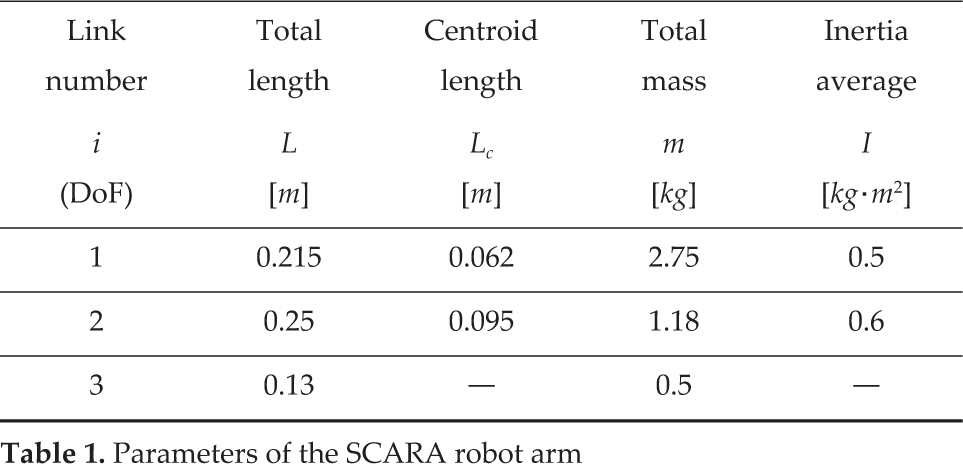
The mechanical configuration of the robot is a three-DoF selective compliant articulated robot for assembly (SCARA) [11] which has first and second joints of revolute type (it allows for the relative rotation between the two links), and linear relative motion can be performed by a third joint of prismatic type. Its parameters are shown in Table 1.
Parameters of the SCARA robot arm
2.1 Direct Kinematics
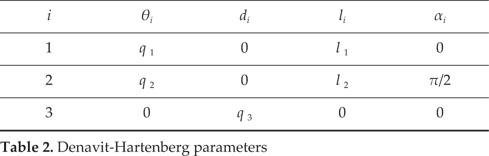
The Denavit-Hartenberg (DH) convention [12] is a commonly used method for selecting frames of reference in robotic plants to obtain a kinematics mathematical model. The DH convention involves the following homogeneous transformation matrix:

where θ, d, l and α are parameters associated with a link and joint i, their values coming from specific aspects of the geometric relationship between two coordinate frames for the specific mechanical configuration of the robot arm;
For a three-DoF robot arm i has three values (1, 2, 3), which must be included in Equation (1), and from which we must obtain three homogeneous transformation matrices (0H1, 1H2 and 2H3). To feed (1) with the values of θ, d, l and α, Table 2 was constructed with the DH parameters of the actual robot.
Denavit-Hartenberg parameters
Now, to go from system 0 to system 3 we compute 0H3 =0H1x1H2x2H3 to obtain the position and orientation of the end-effector using the information of Tables 1 and 2, such that we get:

with
and
where q1 [rad], q2 [rad] and q3 [m] are the articular plant positions.
The direct kinematics for the robot are obtained from the last column of (2) and are given in numerical form as:

where
2.2 Inverse Kinematics
We can obtain the inverse kinematics by solving the Equation (3) for q1, q2 and q3. This can be done including the Moore-Penrose pseudo-inverse Jacobian matrix JT (JJT)−1 in the first time-derivative of q as follows:

where J is the Jacobian matrix obtained from
Computing and integrating (4), the inverse kinematics are obtained and given by:

It can be observed that
2.3 Attitude of the End-effector
The end-effector orientation is given by:

This expression is obtained from Equation (2), which generates a sub-matrix
Considering the parameters of the SCARA arm (Table 1), the solution to (6) gives
2.4 Dynamics
By using the Euler-Lagrange approach [15], a total torque vector

where
Introducing the matrix 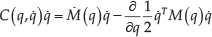


In order to have a numerical dynamics model of the actual robot, we will convert (7) into the following seven-step algorithm taking data from Table 1:
To obtain the forward kinematics for each centroid joint using Equation (3).
To obtain the linear speed v from:

To obtain the kinetic energy (K) present in each i-th link via computing

To obtain the potential energy (U) by Ui (q)=migL cihi where g = 9.81m/s2 and hi are the height of the i-th link.
To obtain the Lagrangian (L) with
To apply the Euler-Lagrange movement equations to obtain the i-th link torque as:

To rearrange the entire resulting expression according to the form that possesses Equation (8). After this, we have:

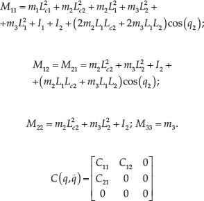


Finally, substituting the parameters of Table 1 we know the numerical values for M, C, 
2.5 State Space Representation
The dynamics equation in the state space is given by:

The function of the robot's mathematical model in a control system implemented in the simulation stage is to have an identifiable pattern for the dual-RNN and to obtain closed-loop results.
3. Dual-RNN
The identification process is required when a control law such as the NBC transformation form needs the appropriate plant model.
The function of the NN within the system is to identify the dynamic plant behaviour. The problem with neural identification is to select an appropriate model for the task as well as the adjustment of its parameters according to some adaptive law so that the response of the neuronal identifier to an input signal approximates the system response for the same input [16].
3.1 Dual-RNN Structure
The dual-RNN is composed of two RNNs - one of them is a first-order RNN and the other is a second-order RNN-both working simultaneously and competing with each other to obtain the best identification values, which are selected by a switching system and according to certain criteria.
Each of the RNNs has a similar structure to that of the state space representation for the robot's dynamic model (see Equation (9)) and they are given in decoupled form by:

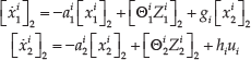
where [·]1 represents a variable or a function coming from the first-order RNN; [·]2 represents a variable or a function coming from the second-order RNN; x1
i
are the NN first-block states which estimate the angular position for the plant; x2
i
are the NN second-block states which estimate the angular velocity for the plant;
It is important to mention that a dual-RNN given by equations (10) and (11) absorbs non-modelled dynamics, parametric variations, system noise and external perturbations through the ΘiZ i product, as well as that the control signal u indirectly affects the first-block states.
3.2 Neural Activation Functions
If equations (10) and (11) represent a dynamic NN and have vectorial activation functions given by
The best activation functions obtained for the first-order RNN are as follows:
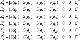
and the best activation functions obtained for the second-order RNN are as follows:
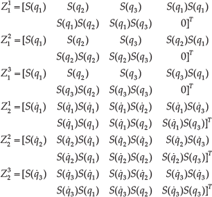
where S (·) represents the tanh (·) function whose products give the second RNN its character as second-order.
3.3 RHONN Training Algorithm
Consider the system described as follows:

where Θ l is the estimator of the NN synaptic weights Θ l ,xl represents the plant states and xl the NN identifier. The difference between both is the identification error, represented as:

being due to meet:

Next, the NN synaptic weights are updated by the training law:

which is called the ‘filtered error algorithm’ [17], where γ represents a learning rate (i.e., an adaptive gain). On the one hand, a very high rate of learning will make the system unstable. On the other hand, a very low rate of learning will make the system slow to learn. This last parameter is obtained in a heuristic way.
To train (10)–(11) l = 1- 6, (15) can be expressed as:

and (17) can be expressed as:

with i = 1,2,3, j = 1,2 and taking into account that
Through Θ, χ becomes an indirect input for the dual-RNN.
3.4 Switching System
The information delivered to the control law (which is discussed in the next section) from the identifier is:
In this work, a novel criterion to select the best values is proposed: take the data coming from the minimum standard deviation of the identification error, expressed by the following laws for switching:
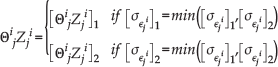

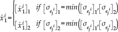
where
Each i,j-th switch acts independently. As such, the dual-RNN output contains information from both the first-order and the second-order RNNs simultaneously. This ensures that the identification process significantly improves, i.e., the dual-RNN identification error (18) is lower than that of any single RNN, the obtained synaptic weights are more accurate and the ΘZ term is closer to the sum of the non-modelled dynamics, parametric variations, external perturbations and noise.
4. Control
The dual-RNN (10)–(11) needs a control signal u for its operation. A NBC transformation form generates this u and is an ideal controller for this work due to the fact that the NBC is designed from a block structure, such as that given by Equation (9).
In nonlinear control theory, there already exists an algorithm to construct a NBC with a similar structure to that of (10) or (11), and from which can be built a driver for the system:

where x represents the states of the system; f(x,t) is a function containing a feedback signal; u is the control signal; φ(x,t) is a function that necessarily does not affect the feedback or the system control term. As such, it represents parametric variations, unmodelled dynamics and disturbances affecting the system, which are calculated through (10)–(11) by the product of the synaptic weights 0 and activation functions Z.
Next, since we have an identification system similar to (23) according to the NBC transformation form technique [18], and taking into account that we have a relative degree system r=2, the following expression is obtained:
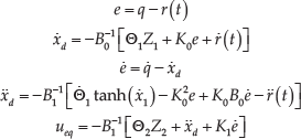
where
The dual-RNN is fed with:

with upper limits of +24 Nm and lower limits of −24 Nm, which are the operational ranges of the plant. The saturation function in (25) acts as a conventional SM.
5. Simulation
The implementation of the system is made in MATLAB-Simulink (Copyrights and registered trademarks of The MathWorks, Inc).
A block diagram was constructed, as shown in Figure 1, to obtain simulation results for the experiments designed in this work.
5.1 Simulation Conditions
For the block model made in Simulink, we have work conditions, listed below.
Equations (10)–(11) and (19) are involved in the subsystem dual-RNN of Figure 1, with the following conditions and parameters:
Neural adaptive gains in the order of 5 × 10⁶ (γ l in (19)).
Feedback gains in the order of unity.
Initial conditions for the NN at the origin.
Computer sampling time is 0.0001 s.
Computer solver: Bogacki-Shampine.
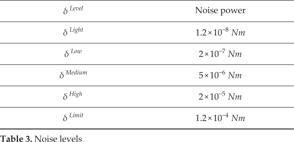
In (9), δ(t) is defined as the system noise and external perturbations. For simulation purposes, let us define δ
Level
with Level = Light, Low Medium, High, Limit as a band-limited white noise function, with a computer sampling time of 0.0005 s, and whose values are given in Table 3 (any seed for the white noise function works out). Moreover, define η (t 0, t 1) as the external perturbation induced by a torque value of t in Nm from the initial time t0[s] to the final time t1[s]. Accordingly,
Noise levels
We should not confuse units for the noise power or the perturbation torque with units of
In what follows, we considered the notation for the initial conditions of the robot as
For the motor moving the third link of the robot, 1 rad is equivalent to 1.9times10-2m of prismatic displacement. For convenience, in this section q3 and
5.2 Simulation Results I
It is important to observe the behaviour of the standard deviation for the identification error (σ∊), since this is the criteria to select the best identification data.
The reference signal r(t) that must track the robot arm in the experiments of Simulation Results I and II is disclosed in Table 4.
Reference signals to track for subsections 5.2 and 5.3

Figures 3–8 show

σ∊ for the first state of the first block
Several operating conditions for the simulation were taken into account, as specified below.
In Figure 3 can be seen
In Figure 4 can be seen

σ∊ for the second state of the first block
In Figure 5 can be seen

σ∊ for the third state of the first block
In Figure 6 can be seen

σ∊ for the first state of the second block
In Figure 7 can be seen

σ∊ for the second state of the second block
In Figure 8 can be seen

σ∊ for the third state of the third block
For all the Figures, every time there is an intersection of lines there is a switching in the output data of the dual-RNN.
In the long run, there is a clear gap between the two lines due to the feedback effect on the dual-RNN. However, the movements of an industrial robot, take less than a second for pick and place processes, welding processes, among others.
5.3 Simulation Results II
To verify the best performance of the dual-RNN with respect to a traditional RNN, is necessary to replace the dual-RNN block in Figure 1 with RNN1 or RNN2, and so obtain results for each in a separate manner. This ensures that the feedback of either one of them does not affect the performance of the other. Table 5 comprises three sections: the top is for the dual-RNN data, the middle is for the RNN1 data (without feedback from RNN2), and the one below is for the RNN2 data (without feedback from RNN1). The data are obtained for different simulation times and there is an averages row for each, where we can observe that the minimum values correspond with those for the dual-RNN. Due to the foregoing, it follows that the dual-RNN as an identification system gives better performance than a single first- or second-order RNN.

5.4 Simulation Results III
The dual-RNN as identifier for the robot arm must adjust the synaptic weights online to obtain the correct neural states: x11,2,3 are the states for the position and x21,2,3 are the states for the velocity. At any given moment, the robot has its own position and joint velocity represented by q123 and
The reference signal r(t) that must track the robot in the experiments of this subsection is shown in Table 6.
Reference signals for Simulation Results III

The first link is working with δ(t)=δ Light + η0(0,0) and χ11(0)=-π/2 [rad, and the results for this identification process are given by Figures 9 and 10. In Figure 9, it is not possible to distinguish between the two lines because, with a light noise level, x11 tracks q 1 in a nearly perfect way. Figure 10 is a zoomed view of the transient of Figure 9, where the ending of the transient before 0.015 s can be seen, which indicates a nearly immediate identification for the first state.

The dual-RNN tracking the robot movements for the first link working with light noise levels

Zoomed view of the transient of Figure 9
The second link is working with δ(t)=δ Medium + η0(0,0) and χ12(0)=-π/2 [rad], and the results for this identification process are given by Figures 11 and 12. It is now possible to distinguish the two lines (the state of the robot (q2) in blue and the state of the identifier (x12) in green). This is due to the medium noise level, which has a noise power near to δ light x400. Nevertheless, as can be seen in Figure 12, the identification time is similar to that with a light noise level. Even more, after the transient the two lines remain attached each other.

The dual-RNN tracking the robot movements for the second link working with medium noise levels

Zoom into the transient of Figure 11
The third link is working with δ(t)=δ Limit + η0(0,0) and χ13(0)=-π/2 [rad], and the results for this identification process are given by Figure 13, where one can see the effect of a strong noise level when positioning the robot. Even so, the dual-NN tries to adjust to the movements of the robot and the identification process is not lost. It is worth mentioning that δ Limit =δ Light × 10000.
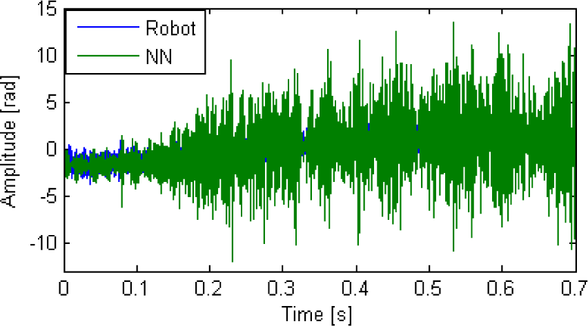
The dual-RNN tracking the robot movements for the third link working with extra-high noise levels
5.5 Additional Results I
With the aim of demonstrating the performance of the control system, tracking results are presented. It is not intended to show the benefits of the driver.
In Figure 14, the second link is tracking the reference signal given in Table 4 with δ(t)=δ High + η1.5(3,3.5), and χ12(0) = π/9[rad]
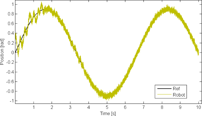
Tracking the reference signal under high levels of noise
In Figure 15, the second link is tracking the reference signal given in Table 4 with δ(t)=δ Low +η0(0,0), and χ12(0)=π/9 [rad].
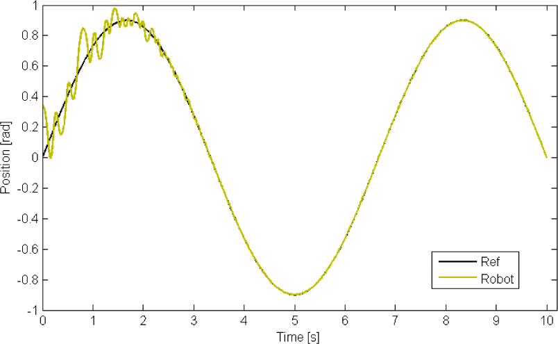
Tracking the reference signal under low levels of noise
It can be seen that the identification process is more difficult for the operating conditions shown in Figure 14 compared to those shown in Figure 15, since with high noise levels the robot's movements are rougher.
5.6 Additional Results II
Even though the aim of this work is not to present the benefits of any control system, in order to give the reader a point of comparison regarding the performance of the dual-RNN operating within the control system, we provide below a performance comparison of the system given in Figure 1 (hereinafter called ‘dual-CS’) against a classic, but enhanced, PID controller, the parameters of which are given in Table 7 and which is tuned heuristically. This enhanced PID controller generates a control signal from a high speed computed control system, which makes it a kind of computed torque control system. For a classic non-enhanced PID, it is virtually impossible to track hard reference signals combined with the highly nonlinear dynamics of the plant.
Proportional, integral and derivative gains for the PID controller

The noise conditions under which the experiments are performed in this subsection are δ Medium and the reference signal r(t) that must track the robot arm is disclosed in Table 8.
Reference signals for Additional Results II

Figure 16 shows the performance of the dual-CS in tracking a square wave as the reference signal. Here, one can observe excellent controller behaviour, even with a medium noise level. Nevertheless, due to the noise - suddenly, for short periods of time - strange behaviour is exhibited in the signal tracking (see in the vicinity of 0.5 s and 8.5 s).

The dual-CS tracking a square wave
Figure 17 shows the performance of the PID controller defined by the first row of Table 7 tracking the same reference signal of Figure 16. It can be seen that the noise does not allow the controller to produce the characteristic PID tracking form for a square wave, which is the same as that produced for a step as the reference signal (a soft rounded overshoot no longer than 25% of the amplitude).

The PID controller tracking a square wave
As occurs in Figure 16, strange behaviour is exhibited in the signal tracking (see in the vicinity of 0.5 s, 2.2 s and 6.2 s).
Figure 18 shows the performance of the dual-CS tracking a sawtooth as the reference signal. As in Figure 16, the dual-CS's performance is remarkable. This kind of reference signal does not produce strange movement for the robot positioning. The return from the overshoot is excellent and the transient is short enough.
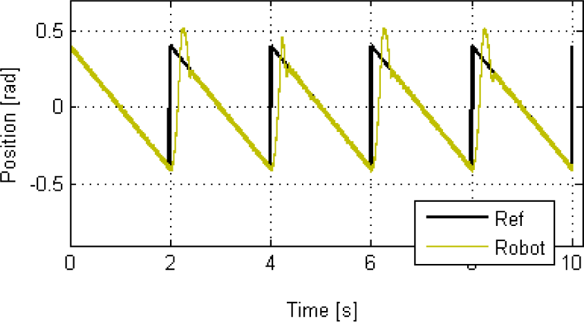
The dual-CS tracking a sawtooth
Figure 19 shows the performance of the PID controller defined by the second row of Table 7 tracking the same reference signal of Figure 18. It can be seen that the controller cannot deal with the noise level, with this kind of reference signal nor with the first and third link movements acting as external perturbations for the second link.

The PID controller tracking a sawtooth
Figure 20 shows the performance of the dual-CS tracking a vectorial sequence as the reference signal. Conclusions for this result are similar to those of Figures 16 and 18, but we can add to the above that do not exist an overshoot when changing the ramp slope (see for 1 s, 3.5 s and 6 s).
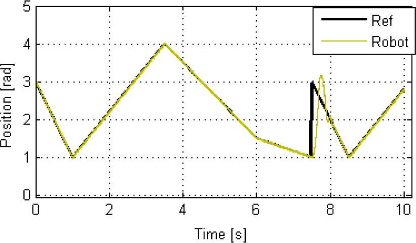
The dual-CS tracking a vectorial sequence
Figure 21 shows the performance of the PID controller defined by the third row of Table 7 tracking the same reference signal of Figure 20. Conclusions are similar to those of Figures 17 and 19 and it can be seen that after 7.5 s the control is lost.

The PID controller tracking a vectorial sequence
6. Conclusions
The dual-RNN is capable of working under different operating conditions, such as strong, high, medium, low and light noise levels, bounded external perturbations and initial conditions for the robot out from the origin.
When a RNN inside the dual-RNN fails to identify, the other RNN becomes the backup for the system (see Figure 5).
The dual-RNN's performance was better than that of a traditional single RNN (see Table 5); as such, this novel dual-RNN becomes an improved identifier for a robot arm.
Furthermore, the dual-RNN gives more robustness to the control system than would be the case for a single RNN.
The authors would recommend the implementation of the dual-RNN if you have a robotic system working inside a factory or a noisy environment, as well as when the tasks of the robot include high-speed or short movements, such as pick and place or welding processes.
The dual-CS, which uses the dual-RNN as an identifier, is stronger and more robust compared with a classical PID controller, both working within similar conditions: the same reference signal and the same noise levels. The use of the dual-RNN is not limited by working within a dual-CS but can be the identifier for any control system that requires it.
Footnotes
7. Acknowledgements
This work was supported by the Consejo Nacional de Ciencia y Tecnología (CONACYT) (México) under scholarship number 248997-307439 with support 000031 and by the Retention Programme 120489.
Special tanks to CONACYT, and Centro Universitario de los Lagos, Universidad de Guadalajara.