
Abstract
This work is concerned with the task space impedance control of a robot driven through a multi-stage nonlinear flexible transmission system. Specifically, a two degrees-of-freedom cable pulley-driven flexible-joint robot is considered. Realistic modelling of the system is developed within the bond graph modelling framework. The model captures the nonlinear compliance behaviour of the multi-stage cable pulley transmission system, the spring effect of the augmented counterbalancing mechanism, the major loss throughout the system elements, and the typical inertial dynamics of the robot. Next, a task space impedance controller based on limited information about the angle and the current of the motors is designed. The motor current is used to infer the transmitted torque, by which the motor inertia may be modulated. The motor angle is employed to estimate the stationary distal robot link angle and the robot joint velocity. They are used in the controller to generate the desired damping force and to shape the potential energy of the flexible joint robot system to the desired configuration. Simulation and experimental results of the controlled system signify the competency of the proposed control law.
Keywords
1. Introduction
Impedance plays an important role in the performance of tasks by manipulators that require interaction with the environment [1]. For example, a laparoscopic surgical robotic system, such as [2], typically works inside the human abdomen, packed with vital organs of which their precise location and geometry are not known. The motion of the forceps is controlled and supervised by a skilful surgeon. Nevertheless, erroneous motion is possible, as a result of which the surrounding organs may be injured. If the forceps are equipped with proper compliance, the severity of wounds can be mitigated. As another example, a service robot system, such as [3], among the others, is able to perform general daily tasks. It is inevitable that such a robot has limited and imprecise information about the environment it interacts with. To successfully implement tasks, the robot must possess appropriate compliance characteristics. A specific impedance model implemented through the mass, spring and damping parameters is popular among the more general functions between the motion and force variables. This representation is intuitive to the human operator and it may be used to shape the behaviour of wheeled inverted pendulum vehicles for better riding experiences [4].
Many efforts have been made in shaping robot compliance to the desired values. However, only a few works have attempted to control the impedance of flexible joint robots. [5] presented a simplified model of a flexible joint robot on which most of the proposed controllers, such as [6] and [7], are based. A tracking impedance controller for the DLR-II arm [8] was proposed using singular perturbation analysis. In contrast, [9] applied a passivity analysis to design a robust and stable impedance control law. Recently, an adaptive impedance controller based on the function approximation technique (FAT) [10] was applied to a flexible joint robot system with motor dynamics included. Impedance behaviour may also be acquired indirectly through admittance control by generating the reference motion from the interaction force error. This idea is applied using an adaptive fuzzy control technique to manipulate the non-rigid environment of the multiple mobile manipulators [11].
The contribution of this research is a passive task space impedance controller for a flexible joint robot system driven through multi-stage nonlinear flexible transmission based only on the motor angle signal. Motor current feedback may optionally be used to improve the system response time. In particular, an embodiment of a prototypical two degrees-of-freedom (DOF) cable pulley-driven flexible joint robot is investigated. Section 2 develops the detailed model of the robot, its counterbalance and its flexible drivetrain subsystems. A model of the complete system is then obtained by integrating these together using the bond graph framework. Based on this model and the available feedback signals of the motor current and angle, in section 3 a task space impedance controller is designed to accomplish the desired viscoelastic behaviour at the specified set point. The stability of the closed-loop system is proven. In order to validate the effectiveness of the control law, various simulations and experiments of the system are conducted and the results are discussed accordingly in section 4. Finally, section 5 concludes the study.
2. System Modelling
A two-DOF cable pulley-driven flexible joint robot, shown in Figure 1, is constructed as a prototype serving as a fundamental study of the multi-stage cable pulley-driven robot class, which will further be employed in developing the entire arm of our ongoing service robot project. It comprises three subsystems, namely a rigid robot, a flexible transmission and a counterbalance. The robot shoulder link is capable of moving in the pitch and yaw directions, emulating the principal motion performed by the human shoulder. Generalized coordinates describing the position of its end-tip may naturally be chosen as the pitch and yaw angles, denoted as

A two-DOF multi-stage cable pulley-driven flexible joint robot
Figure 2 depicts the winch and pulley arrangement of the robot's multi-stage transmission subsystem. Starting from the input side, the motor axle is coupled to winch#1, which then drives winch#2 through the wrapped cables. Winch#2 in turn drives pulley#1 (for the right winch) and pulley#2 (for the left winch). Together with pulley#3, these pulleys form the differential mechanism which produces the rotational motion of the output shoulder link around two mutually perpendicular axes, causing the motion of the shoulder link end-tip in the pitch and yaw directions. A differential mechanism is implemented in this work through the cables and stepped pulleys. In addition, the additional pulley#4 is not attached to any cable – its purpose is to counter pulley#3 and to strengthen the structure.

Winch and pulley arrangement in the drivetrain unit of the flexible joint robot. Left winch#1 is occluded.
Furthermore, the robot is equipped with a patented (pending) counterbalancing mechanism [12], invented to reduce the amount of torque commonly required by the motors to sustain weight and, hence, to improve the safety of the robot. Basically, the motions of pulley#1 and pulley#2 are transmitted via the cable routing to elongate a set of springs. With an appropriate spring stiffness selected, the generated torque can match the configuration-dependent gravitational torque. Such considerations may apply from the viewpoint of maintaining the total potential energy of the system.
2.1. The Robot System
Referring to Figure 2, the position vector of the shoulder link end-point relative to the origin of
For the spherical configuration of the robot, the velocity of the end point may be determined simply from the fact that its motion comprises pure rotation around the origin of the fixed frame

The main moving parts of the robot are pulley#3, pulley#4 and the output shoulder link. For convenience, the rectangular frame of the counterbalancing mechanism subject to the pitch motion will be included as well. These components may be grouped into two categories: one undergoing pitching motion alone, and the other undergoing a composite pitching and yawing motion. CAD drawings of these two collections are depicted in Figure 3. Their related parameters will thus be subscripted as ‘p’ and‘

(left) Collection of mechanical parts undergoing pitching motion. (right) Collection of mechanical parts undergoing pitching and yawing motion.
For the first collection undergoing pitching motion, its compound centre of gravity (C.G.) is evaluated by the CAD program to be at

where

for which
Similarly, the kinetic and potential energy of the pitch/yaw collection may be derived as follows. From the geometry, the compound C.G. location is at

for which the careful design of the shape of the parts makes the off-diagonal elements of the inertia matrix

with
Robot parameter values

2.2. The Counterbalance System
The counterbalancing mechanism contributes to the robot dynamics by maintaining the constant potential energy of the augmented system. The mechanism may be divided into two parts. Figure 4 illustrates a part of the mechanism [12] where the cable (20) is routed through the set of idlers (21-24) to convey the tension force from the spring (12) to the stud (18) embedded in pulley#2. The generated torque will counter the gravitational torque of the pitch/yaw collection. The other simple part of the mechanism accounts for the pitch-collection. Note that, due to the (generally) non-zero initial tension of the spring, the cable routing over non-zero radius idlers and the travelling limitation hit of the mechanism, the compensator departs from theory. Nevertheless, the current consumption of the motor in holding the robot statically is reduced dramatically; the current is now bounded within the band of ±0.1 [A] as compared with the average value of 1.5 [A], when there is no assistance from the counterbalance.
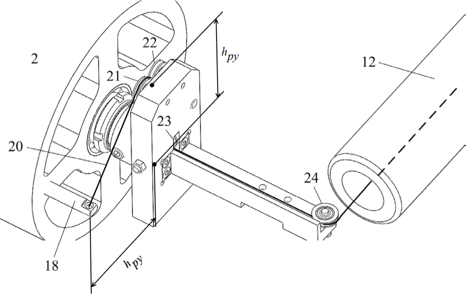
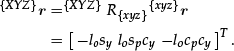
Counterbalancing mechanism for the pitch/yaw collection of the robot [12]. The shortest distance of the cable terminal at pulley#2 measured from the X – X axis,
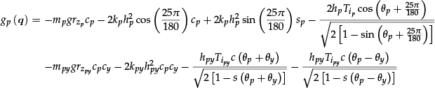
The force and induced moment produced by the mechanism may be analysed indirectly via the spring potential energy of the counterbalance. The cabling of the mechanism enforces the elongated length of the springs in relation to the robot configuration through its generalized coordinates
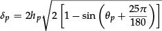

where

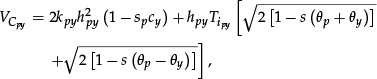
in which


Additionally, the friction force
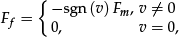
where v is the signed velocity of the slider and
According to the above energy analysis, the Lagrangian of the robot plus its counterbalances may be determined as:

where

with:

Parameter values of the counterbalancing mechanism

In Eq. 15,

The external force caused by the robot interacting with the environment at the end of the shoulder link may naturally be described in the task space frame as

as can also be verified by inspecting the robot geometry directly. Finally,
2.3. The Transmission System
The pulley and winch arrangement of the multi-stage flexible transmission is illustrated in Figure 2. It can be seen that the drivetrain is designed to have four stages for compactness. In the
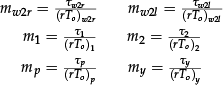
Let
This particular system is designed such that the transmission ratio, n, at the
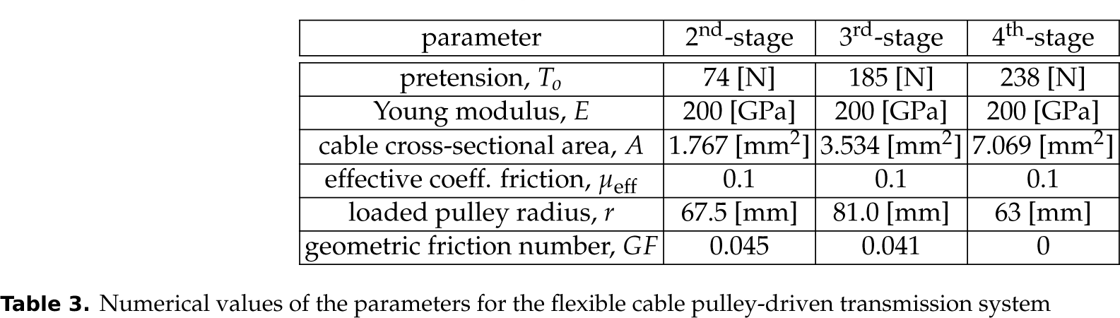
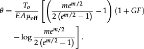
Since the mechanism employs the cables as the means for transmitting power, its inherent compliance characteristics should be taken into account. Assuming the cables have been securely wrapped around the pulleys with proper pretension, such that the total slippage between the cable and the pulley groove over the circuit is negligible, the explicit torque-angle deflection equation of a stiff simple cable pulley drive unit may be determined [13] as:

where the cable, with a Young modulus E and an effective cross-sectional area A, has been pre-tensioned to
Numerical values of the parameters for the flexible cable pulley-driven transmission system
The compliance analysis in [13] can be extended to handle the cable pulley differential mechanism at the
In this case, m is the dimensionless torque of the loaded torque M applied along the pitch or yaw directions. Since there is no unwrapped segment of the cable for the differential drive unit, effectively
Major loss in transmission happens at the bearing units. The complexity of the friction phenomenon at the support leads us to propose a friction model as a combination of the simple Coulomb's friction torque when the relative velocity of the mating surfaces is virtually zero, and the empirical formulation of the frictional torque for the standard sealed deep-grooved ball bearing [14] when relative motion occurs. Mathematically:

where

Detailed bond graph diagram of the two-DOF cable pulley-driven flexible joint robot-controlled system. The diagram displays the interconnection of the controller, motor, drivetrain, counterbalance and robot subsystems. The physical system-like couplings of the lumped model of the system's components ease the understanding of the overall dynamics.
Shaft diameter and pulley radius values in [mm] at each rotor-bearing support
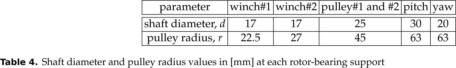
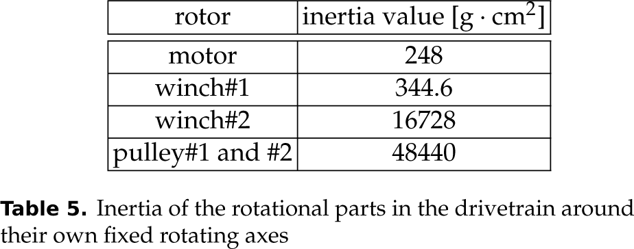
The inertias of the rotational parts in the transmission unit are summarized in Table 5. Hence, the complete dynamics of the drivetrain may now be determined by combining the inertial, the dissipating and the elastic torques according to the system's kinematic configuration, together with the externally applied torque of the motors. Unfortunately, the explicit form of the equations for motion is barely achieved due to the inversion problem of the complicated nonlinear deformation functions in Eqs. 21 and 22. This, however, does not affect the simulation or the control law implementation.
Inertia of the rotational parts in the drivetrain around their own fixed rotating axes
2.4. The Complete System
A realistic model of the two-DOF multi-stage cable pulley-driven flexible joint robot which captures its important behaviours may be acquired through the bond graph technique [15]. With this approach, the system model is constructed by identifying the governing equations of the subsystems, comprising the bond graph basic elements of one-port inertance, compliance, resistance and two-port transformer and gyrator.
Nevertheless, the robot dynamics are modelled using the customized nonlinear two-port inertance and compliance elements. In particular, the equation of motion Eq. 15 is expressed in the Hamiltonian form with the generalized coordinates

All of these elements are then combined through the power bonds and the effort/flow ports. The complete bond graph diagram is given in Figure 5.
3. Task Space Impedance Control
3.1. The Controller
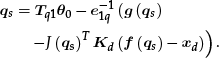
A task space impedance control for the robot driven through a multi-stage nonlinear flexible transmission system has been developed in [16]. The controller uses the available feedback information of merely the motor current and angles, which is frequently encountered in practice. In particular, if the desired task space compliance and dissipative damping ratio,
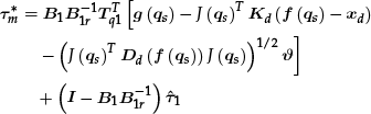
computes the motor reference torque
The controller is based on the estimated stationary robot link angles


The argument s represents the complex argument of the Laplace transform.
The estimated transmitted torque may be achieved by discretizing the motor equation of motion with the variational integrator method [17], which guarantees the energy conservation at every sampling. As a result, the transmitted torque at the
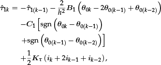
where
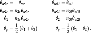
For this two-DOF cable pulley-driven flexible joint robot, Eq. 26 is tailored to:

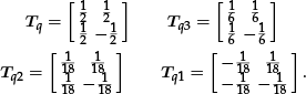
with the following compound transmission ratios:
The individual deformations at each stage are determined from the coupling stiffness and the cable pulley compliance relationship of Eqs. 21 and 22:

where:

are the torque vectors transmitted over the elastic couplings and cable pulley mechanisms to winch#1, winch#2, pulley#1, pulley#2 and the pitch and yaw joints of the robot. Also:
are their dimensionless values.
Nominal control parameters adopted in the simulations and experiments

For this system with the desired task space stiffness matrix

as a function of the stationary robot joint angle
The designed controller is integrated with the developed model of the two-DOF cable pulley-driven flexible joint robot. Figure 5 depicts the signal interconnection between the system and the controller, where the motor current and angle are fed back to the controller unit to process the commanded current. The controller is digitally implemented at a frequency of 1 kHz. For the simulation, the controller computation is done in MATLAB connected to the 20-sim [18]. This simulation program is based on the bond graph modelling language, which does not require the explicit formulation of the complete system's differential equations. At each sampling,
3.2. Stability of the Closed-loop System
Proof. Before proving the stability of the closed-loop system, let us consider the estimated link joint velocity of Eq. 28. It may be viewed as the stable linear filtering of the time derivative of the estimated link angles
where
Define the new state vector

where the input is now the regulation error
Let
consisting of the kinetic energy (KE) and potential energy (PE) of the robot, the KE of the reduced inertia drivetrain according to its dynamics (rotor inertia matrix

the elastic PE of the drivetrain:
the negative PE of the controller:

and the KE-like function of the velocity estimator unit. According to Eq. 27,

It can be shown that the function
The above equilibrium point

where
the derivative may be simplified to:

The realistic transmission system is fully damped, making
4. Simulations and Experiments
In what follows, various simulations and experiments are performed to investigate the effect of several control parameters on the system response and to illustrate the effectiveness of the control law. Since the system is rather stiff, an adaptive backward differentiation formula integration method with a step size of 1 [ms] is used in all simulations. In the real system, due to the discrete implementation of the controller and the unmodelled dynamics, the achievable desired stiffness and damping ratio are reduced to the values shown in Table 6. Additionally, the motor current has been limited to 3.5 [A] for safety reasons.
4.1. Constant Set Point
Let the initial position of the robot end-point be at the centre of its hemispherical workspace, i.e.,

Motion response of the end point X/Y-coordinates for a constant set point simulation
4.2. Trajectory-tracking
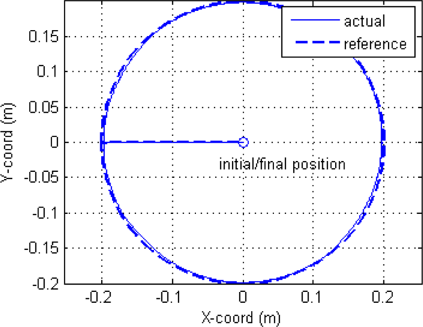
A circular trajectory is generated for the free-tracking simulation. The starting point is at the rightmost,
Figure 7 displays the trajectory-tracking of the robot along with the reference trajectory. It can be seen that the proposed controller – which was designed for the regulation objective – may well be used in the tracking task, since it can tolerate a moderate speed and accuracy. The initial mismatch does not effect the tracking performance or destabilize the system. It merely causes current saturation of the motor during a large position error. Once the end-tip enters its track, the current consumption is quite low (0.45 [A] average) thanks to the energy restoration from the truly passive control of the augmented counterbalancing mechanism.

Simulated trajectory-tracking of the robot with initial position mismatch
A similar experiment is implemented with the real system. The reference trajectory, which may be divided into three parts, starts from the centre point of the robot workspace. Then, it moves leftwards by executing the yaw rotation for
Figure 8 displayed the estimated stationary path of the robot end-tip and its reference. It is seen that the actual robot motion tracks the desired trajectory faithfully. The average of the integral of the absolute error
Circular trajectory-tracking of the real system under no external force
4.3. Task Space Stiffness and Damping
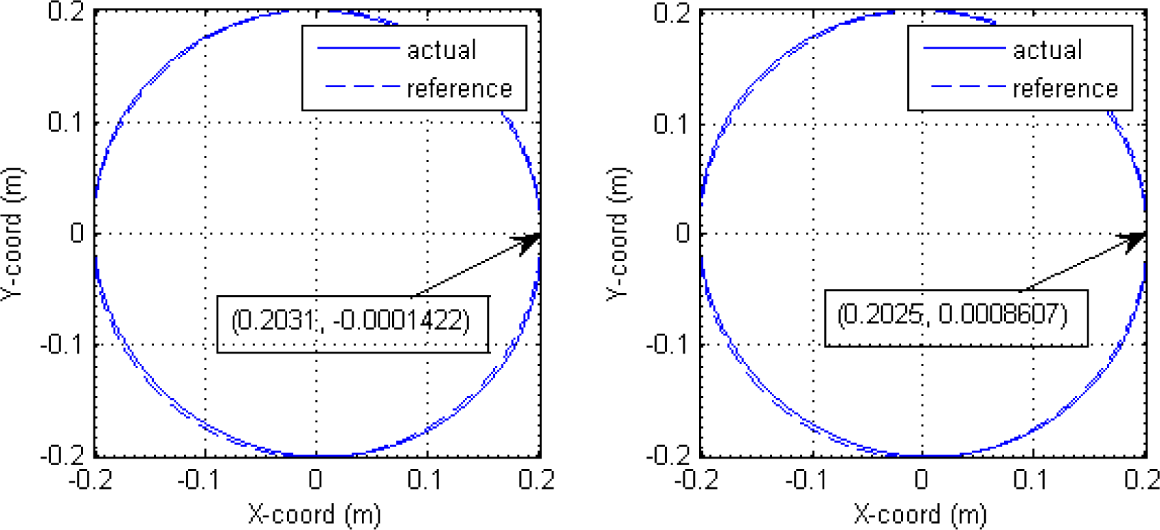
To verify that the desired task space stiffness is actually achieved, the robot is set at the centre of the workspace and an external force of 10 [N] is applied in the X- and Y-directions, respectively. For the simulation, the end-tip deflection responses using the nominal stiffness value are shown in Figure 9 for a set of damping ratios of 0.8, 1.0, 2.0 and 4.0. It is observed that, in practice, increased damping makes the motion more sluggish, while the current drawn (not shown) becomes more responsive. Together with a larger stiffness (order of

Simulation of the robot end-tip deflection with the nominal stiffness value subject to the external force of 10 [N] for a set of damping ratios
Figure 10 and 11 show the deflection plots for stiffness values of 1000 and 100,000 [N/m]. A lower stiffness with high damping causes the end-tip to deflect slowly and prevents it from reaching the expected deviation. Subsequently, the environment will feel the robot become stiffer than its actual value. The deflection of the system with high stiffness and light damping will largely oscillate around the steady value long before it dies out. On the other hand, if too high a damping ratio is selected, the responsive motor current will suppress the deflection aggressively such that the undershoot may be detected. If the damping is further increased, it can cause the system to become unstable.

Simulation of the robot end-tip deflection with a stiffness value of 1000 [N/m] subject to an external force of 10 [N] for a set of damping ratios
Simulation of the robot end-tip deflection with a stiffness value of 100,000 [N/m] subject to an external force of 10 [N] for a set of damping ratios. The system will be unstable if a ratio value of 4.0 or higher is used.
For the actual system, a proof mass of 1.0 [kg] is placed at the end of the robot shoulder link to realize a constant external force in the negative Y-direction, as illustrated in Figure 12. A set of stiffness and damping ratio values, as depicted in Table 7, are tuned to perform the experiment. Figure 13 depicts the estimated end-tip deflections with different impedances. The responses of the real system agree with the simulation results. The static position of the robot end-tip is measured by a vernier height gauge (0.02 [mm] of resolution) before and after applying the weight to obtain the actual deflection value, as recorded in Table 7. Using the commanded stiffness and the estimated stationary pitch and yaw angles, the predicted deflection may be determined from Eqs. 41 and 42. It is observed that the actual deflection is less than the predicted value. This is due to the friction in the mechanism, which causes the effective stiffness to be higher than the desired value.

Robot setup for experiments with varying end-tip stiffnesses and damping values

Static deflection of the robot end point subject to 1.0 [kg] deadweight with different compliance behaviours
Actual responses of the robot end tip deflection subject to 1.0 [kg] deadweight

It should be mentioned that motor inertia reduction will increase the effective stiffness, since it has the effect of increasing the control loop gain and thus the resultant stiffness becomes larger than the desired value. Therefore, motor inertia reduction should not be implemented if the exact desired stiffness is of concern.
4.4. Application of an External Force
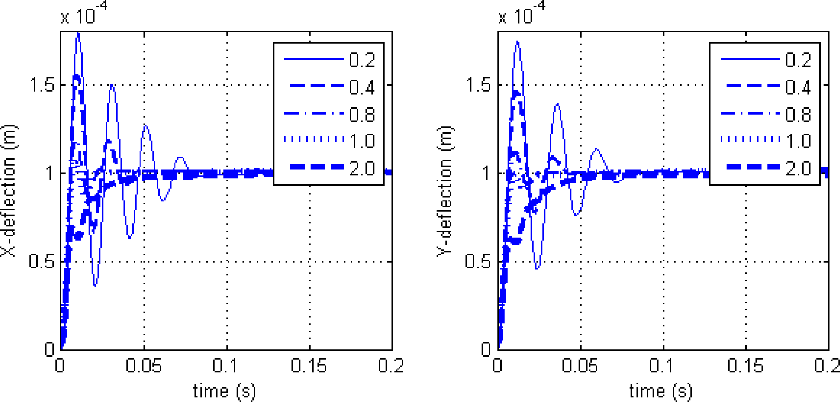
For the last experiment, an external force is applied to the end point while the robot is tracking the same trajectory as in subsection 4.2. The task space stiffness and damping ratio are set to their nominal values. Figure 14 displays the tracking simulation result when the robot is subject to the 10 [N] force acting in the X- and Y-directions throughout the circular path. It was observed that the end-tip follows the reference trajectory closely because of the high stiffness value compared to the magnitude of the applied force. As depicted in the figure, ultimately the end-point deviates from the desired location by 0.6 and 0.86 [mm] along the X- and Y-directions respectively.
Tracking simulation with nominal stiffness subject to a 10 [N] force applied along the X – (left) and Y – (right) directions
When the end-point is at its final position, the nominal task space stiffness matrix expressed in the local frame parallel to the reference frame

where the numerical value of

along the direction of the applied force will be 0.59 and 1.0 [mm] for each case in turn. Hence, the actual deviations agree with the theoretical values with only a slight mismatch because of friction. Therefore, the desired end-effector stiffness is achieved.
The tracking result of the real system with a constant force in a negative Y -direction supplied by the attached 1.0 [kg] deadweight is depicted in Figure 15. Due to a weaker nominal stiffness value, the actual motion deviates more from the reference path. Following tracking, the end-point departs from the workspace centre by −0.0176 [m] along the Y -direction while the predicted value is −0.0196 [m]. This agrees with the result in the previous subsection. The tracking performance via the average of the integral of absolute error is 0.0168 [m], which is approximately 2.5 times larger than that of the free-tracking case. The current consumption during the course is plotted in Figure 16. The average values are 2.05 and 1.87 [A] for the right and left motors respectively. From the graph, both motors are saturated for a short period during tracking. It should be noted that the controller exhibits robustness in relation to the unmodelled inertia of the deadweight.

Trajectory-tracking of the real system subject to 1.0 [kg] deadweight at the end-tip

Motor current consumption during circular path-tracking subject to 1.0 [kg] deadweight
5. Conclusions
A prototypical system of a two-DOF cable pulley-driven flexible joint robot is designed and analysed. Important characteristics of the system components are modelled using the Lagrangian energy method. They are organized and integrated using the bond graph modelling technique to accomplish a realistic model of the whole system. A task space impedance controller for a robot driven through a multi-stage nonlinear flexible transmission system is proposed. This regulates the stiffness and damping of the end-effector at the specified position in accordance with the desired values based on just the motor current and angle feedback. The stability of the overall system is proven.
From the simulation, the controller exhibits satisfactory results for standard tasks, such as regulation or trajectory-tracking, both with and without the application of external force. An additional simulation is performed to verify that the specified task space stiffness is indeed achieved. The effects of the damping ratio value on the motion response are studied. Overly high stiffness and light damping cause the robot to oscillate significantly before settling down. On the other hand, the robot moves sluggishly if too low stiffness and high damping are selected. Experiments with the real system further ensure the simulation results. From the investigation, it is evident that the proposed controller is capable of regulating the task space impedance of the manipulator coupling with a multi-stage nonlinear flexible transmission unit in a stable and robust manner. This development will be of great benefit to advanced manipulators in accomplishing challenging missions amidst complex environments.
Footnotes
6. Acknowledgements
The author is grateful for the generous support from many sources, including the Ratchadaphiseksomphot Endowment Fund of Chulalongkorn University (RES560530224-AS), the Thailand Research Fund (MRG5580227 and MSD56I0018), the ISUZU Research Foundation, and the Department of Mechanical Engineering, Chulalongkorn University.