
Abstract
This paper presents the isotropic placement of multiple optical mice for the velocity estimation of a mobile robot. It is assumed that there can be positional restriction on the installation of optical mice at the bottom of a mobile robot. First, the velocity kinematics of a mobile robot with an array of optical mice is obtained and the resulting Jacobian matrix is analysed symbolically. Second, the isotropic, anisotropic and singular optical mouse placements are identified, along with the corresponding characteristic lengths. Third, the least squares mobile robot velocity estimation from the noisy optical mouse velocity measurements is discussed. Finally, simulation results for several different placements of three optical mice are given.
Keywords
Introduction
For the velocity estimation of a mobile robot, several attempts have been made to use optical mice that were originally invented as an advanced computer pointing device [1–11]. In fact, an optical mouse is an inexpensive but high performance motion detection sensor with a sophisticated image processing engine inside. Optical mice installed at the bottom of a mobile robot, as shown in Figure 1, can detect the motions of a mobile robot traveling over a plane surface. Mobile robot velocity estimation using optical mice does not suffer from the problems of typical sensors: wheel slip in encoders, the line of sight in ultrasonic sensors and heavy computation in cameras.

A prototype of a three optical mice array for mobile robot velocity estimation [4]
A pair of optical mice was proposed as a simple but viable means for carrying out mobile robot velocity estimation in the presence of wheel slip [1, 2]. Using redundant velocity measurements of two optical mice, a simple procedure for error detection and reduction in the mobile robot velocity estimation was developed [3]. The redundant number of optical mice was proposed to reduce the effect of the noisy velocity measurements of optical mice and to handle their partial malfunction [4]. Using the geometrical relationships between the optical mice, the calibration for systematic errors and the selection of reliable velocity measurements were carried out [5].
For a mobile robot with a circular base, a regular polygonal array of optical mice can be a natural and desirable choice for the placement of the optical mice. For instance, a pair of optical mice is placed so as to be symmetric around the centre of a mobile robot. Furthermore, N(≥ 3) optical mice are placed in a regular N -gonal array, the geometrical centre of which is coincident with the centre of a mobile robot [4]. However, there can be some restrictions on the installation of optical mice, if the mobile robot has a non-circular base or other structures are pre-installed on its base. With positional restriction on installation, a non-regular polygonal array of optical mice can be a better choice, compared with its regular polygonal counterpart [6].
The performance of an optical mouse array for mobile robot velocity estimation can be evaluated based on its Jacobian matrix. The Jacobian matrix maps the velocity of a mobile robot to the velocities of optical mice, which is a function of the installation positions of optical mice. Through the Jacobian matrix, the unit sphere in the optical mouse velocity space can be mapped into an ellipsoid in the mobile robot velocity space. For the optimal placement of optical mice, the volume of the ellipsoid can be one measure and its closeness to a sphere, the so-called isotropy, can be another measure. The concept of isotropy has been adopted for the optimal design of serial and parallel manipulators [7–11], as well as, omnidirectional mobile robots [12, 13].
This paper presents the isotropic placement of optical mice for mobile robot velocity estimation. It is assumed that there can be positional restrictions on the installation of optical mice at the bottom of a mobile robot. This paper is organized as follows. Section 2 obtains the velocity kinematics of a mobile robot equipped with optical mice, and Section 3 analyses the resulting Jacobian matrix symbolically. Sections 4, 5, and 6 identify the isotropic, anisotropic, and singular optical mouse placements, along with the corresponding characteristic lengths. Section 7 discusses the least squares mobile robot velocity estimation from the noisy optical mouse velocity measurements. Section 8 gives the simulation results for several placements of three optical mice. Finally, the conclusions are presented in Section 9
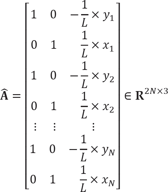
The velocity of a mobile robot traveling on a plane can be estimated using the velocity measurements of N(≥ 2) optical mice installed at the bottom of a mobile robot. Figure 2 shows three coordinate frames that are used for the description of a mobile robot and the ith optical mouse. Let OW, XW, and YW denote the origin, and the x and y axes of the world coordinate frame, respectively; let OR, XR, and YR denote the origin, and the x and y axes of the mobile robot coordinate frame, respectively; and, let Oi, Xi, and Yi, i = 1, ···, N, denote the origin, the x and y axes of the ith optical mouse coordinate frame, respectively. For a simple description, the following assumptions are made. 1) Two origins, OW and OR, are coincident with the centre, denoted by O, of a mobile robot. 2) The origin, Oi, i = 1, ···, N is coincident with the installation position, Pi, of the ith optical mouse. 3) The mobile robot coordinate frame is aligned with the ith optical mouse coordinate frame. The position vector, p i = [xi yi] t , i = 1, ···, N, of the ith optical mouse can be expressed by

Three coordinate frames for a mobile robot and the ith optical mouse

In the above, θ is the angle of rotation of the mobile robot coordinate frame with reference to the world coordinate frame; ρ
i
and ϕ
i
are the polar coordinates of the installation position Pi of the ith optical mouse. Note that the heading angle of a mobile robot is given by
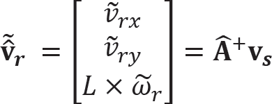
Let vrx and vry be two linear velocity components of a mobile robot along the x axis and the y axis, respectively, and ω r be its angular velocity component around the centre O of a mobile robot. Furthermore, let vix and viy, i = 1, ···, N be the lateral and longitudinal velocity measurements of the ith optical mouse. The velocity relationship between a mobile robot and the ith optical mouse can be presented by


From (2) and (3), the velocity kinematics of a mobile robot with an array of N optical mice can be obtained by [1, 4–6, 14, 16, 17]

In the above,

Note that the expression of
In the velocity kinematics of (4), the velocity vector of a mobile robot,

where
Note that all elements of

where


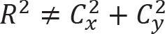
In the above, Cx and Cy, respectively, represent the averages of the x and y coordinates of the position vectors,
or

where


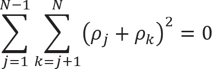
The following inequality relationships exist between the three eigenvalues, λ1, λ2, and λ3 [6]:

In the case of

And, in the case of

Using (18) and (19), from (14) and (15), it follows that λ1 ≥ λ2 (= N), regardless of the values of C
x
, C
y
, and R2, as well as L. Similar to the above, it can be also shown that λ3 ≤ λ2(= N). Note that λ1 and λ3 are the largest and smallest eigenvalues of
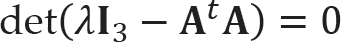
For the 2N × 3 Jacobian matrix

where σ1 and σ3 represent, respectively, the largest and smallest singular values of
The placement of N optical mice is said to be isotropic, if the isotropy of the 2N × 3 Jacobian matrix

for which


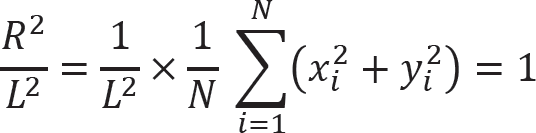
In the above, (22) and (23) indicate that the geometrical centre of N optical mice coincides with the centre O of a mobile robot. Furthermore, (24) indicates that the squared value of the characteristic length should be equal to the average of the squared distances of N optical mice from the centre O of a mobile robot.
Using (1), (22) and (23) can be written as:

Let SN be the isotropic set of the position vectors of N optical mice, satisfying (25):

For given N(≥ 2) optical mice, Figure 3 shows the isotropic sets of N position vectors,
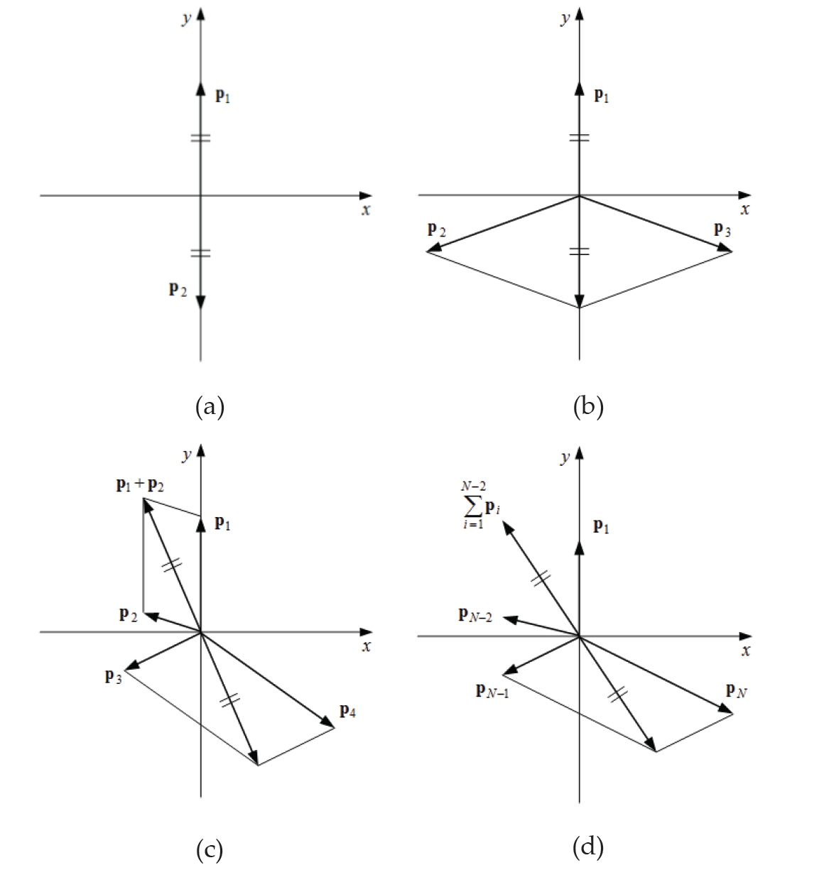
The isotropic set of the position vectors of N optical mice: (a) N = 2, (b) N = 3, (c) N = 4, and (d) N ≥ 4.

where

represents the rotation matrix.
Since the union of two isotropic sets is also isotropic, new isotropic sets for N(≥ 4) position vectors can be obtained from existing isotropic sets known already:
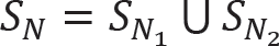
where N = N1 + N2, 2 ≤ N1, N2 ≤ N − 2. For N = 5 optical mice, Figure 4(a) shows the isotropic set S5, which is obtained as the union of S2 and S3. However, note that (29) cannot produce all possible isotropic sets of N position vectors, since


Two isotropic sets of N = 5 position vectors: (a) the union of S2 and S3, and (b) a regular pentagon
Figure 4(b) shows the isotropic placement of N=5 position vectors, which is a regular pentagon.
Once the isotropic placement of N optical mice, denoted by

which is called the optimal characteristic length. Note that the optimal characteristic length L* is the root mean square of the distances of N optical mice from the centre O of a mobile robot.
For a given placement of N optical mice, it may be impossible to achieve the isotropy of the 2N × 3 Jacobian matrix
which is the inverse of the condition number κ of
For the placement of N optical mice, it is desirable to make the value of γ as large as possible. Using (14) and (16), (33) can be written as

with


Differentiating the condition index γ, given by (34), with respect to L, we have

where


Setting

Plugging (35), (36), (38), and (39) into (40), it follows that

As will be shown later,
unless

which results in

which is called the suboptimal characteristic length. It should be noted that the expression of the suboptimal characteristic length L#, given by (44), is the same as that of the optimal characteristic length L*, given by (32).
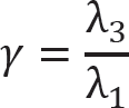
With the suboptimal characteristic length L# known, the maximum value of the condition index γ that can be achieved for a given anisotropic optical mouse placement can be obtained. Plugging (43) and (44) into (35) and (36) and using (34), we obtain

which is called the maximal condition index. Note that the maximal condition index γ# can have values between zero and unity, where γ# = 1 when C
x
= C
y
= 0, and γ# = 0 when
The placement of N optical mice is said to be singular, if

for which the condition index becomes zero, γ = 0. From (16) and (46), we have

which leads to

Plugging (9)–(11) into (48), we have

Using (1), (49) can be written as
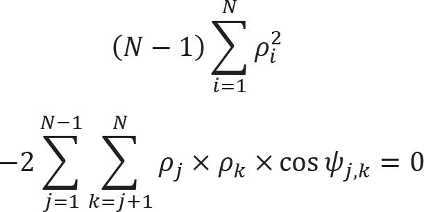
where

represents the angle between two position vectors,
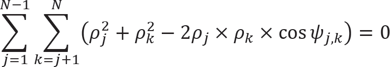
where
Since
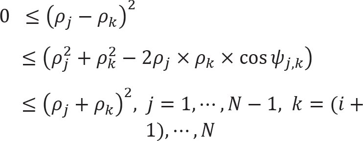
we have

In the above, the equality holds, when
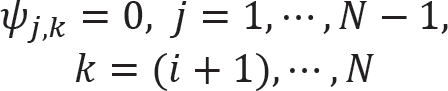
and, from (52), we have

which results in

Note that (55) and (57) indicate that N optical mice are placed at the same position on a mobile robot. Next, in the latter case, for which
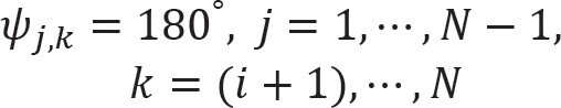
and, from (52), we have
which results in

(60) indicates that N optical mice are placed at the centre O of a mobile robot. At both singular placements of N optical mice, one given by (55) & (57) and the other given by (60), it should be noted that the rank of the Jacobian matrix
Based on the velocity kinematics of (6), the mobile robot velocity can be estimated from the noisy velocity measurements
where

Note that (61) with (62) represents the least squares solution to (6), which minimizes
Let us consider the least square mobile robot velocity estimation, for the isotropic placement of N optical mice, with the isotropic position vectors

Using (63) from (61), three estimated velocity components of a mobile robot are obtained by


where

represents the angular velocity component experienced by the ith optical mouse, which is equivalent to the velocity measurement
Now, let us discuss the role of the characteristic length L in least squares mobile robot velocity estimation, given by (61) with (62), which involves the inversion of
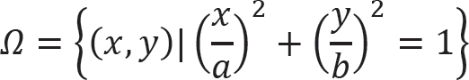
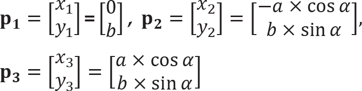
Suppose that three optical mice (N = 3) are placed on an elliptical path, given by
where the first optical mouse is fixed on the principal axis along the y axis, but the second and third optical mice that are symmetric with respect to the y axis, are movable, as shown in Figure 5:

The symmetrical placement of three optical mice along an elliptical path
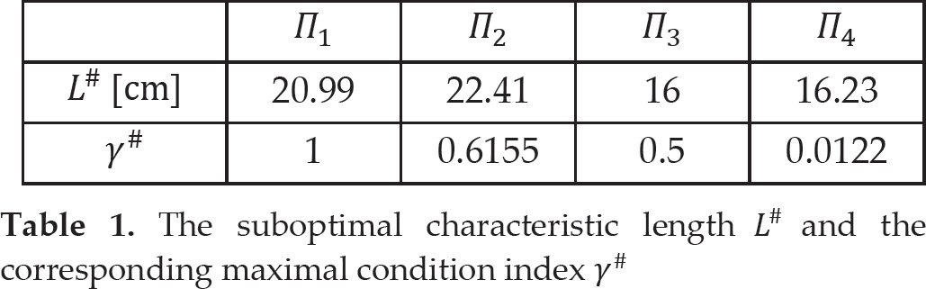
with a = 25 cm, b = 16 cm, and 0° ≤ α ≤ 90°. Using (22) and (23), the isotropic optical mouse placement can be found at α* = 120°, corresponding to ((ϕ1*, ϕ2*, ϕ3*) = (90°, 210°, 330°). Note that three optical mice form an equilateral triangle in general, but they will form a regular triangle if the elliptical path Ω becomes circular, that is, a = b. Furthermore, using (32), the optimal characteristic length is obtained by

shows the changes of the condition index γ, according to the value of the characteristic length L, for four optical mouse placements, Π1, Π2, Π3, and Π4.
The suboptimal characteristic length L# and the corresponding maximal condition index γ#
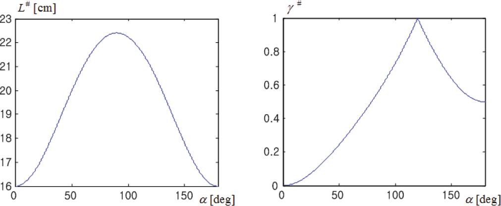
The changes of the suboptimal characteristic length L# and the corresponding maximal condition index γ#, according to the value of the angle α.
Next, let us examine the least squares velocity estimation of a mobile robot for a given placement of three optical mice. Let us assume that a mobile robot is commanded to move forward along the γ axis at a velocity of vrx = 0 cm/sec, vry = 20 cm/sec, and ω
r
= 0 deg/sec. To simulate the noisy velocity measurements of three optical mice, normally distributed random numbers, nix and niy, i = 1,2,3, with mean 0 cm/sec and variance 0.2(cm/sec)2 are added, independently, to the nominal values of the x and y velocity components of each optical mouse. With

where

In the case of the isotropic optical mouse placement Π1, the least squares mobile robot velocity estimation for a linear velocity of a mobile robot: (a) the measured velocity components, v1x and v1y, and (b) the estimated velocity components,
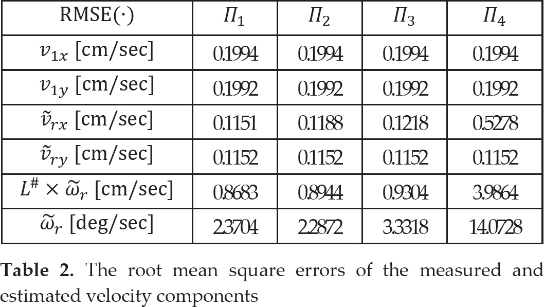
For four optical mouse placements, Π1, Π2, Π3, and Π4, Table 2 lists the root mean square errors of four components of the estimated mobile robot velocity, denoted by
The root mean square errors of the measured and estimated velocity components
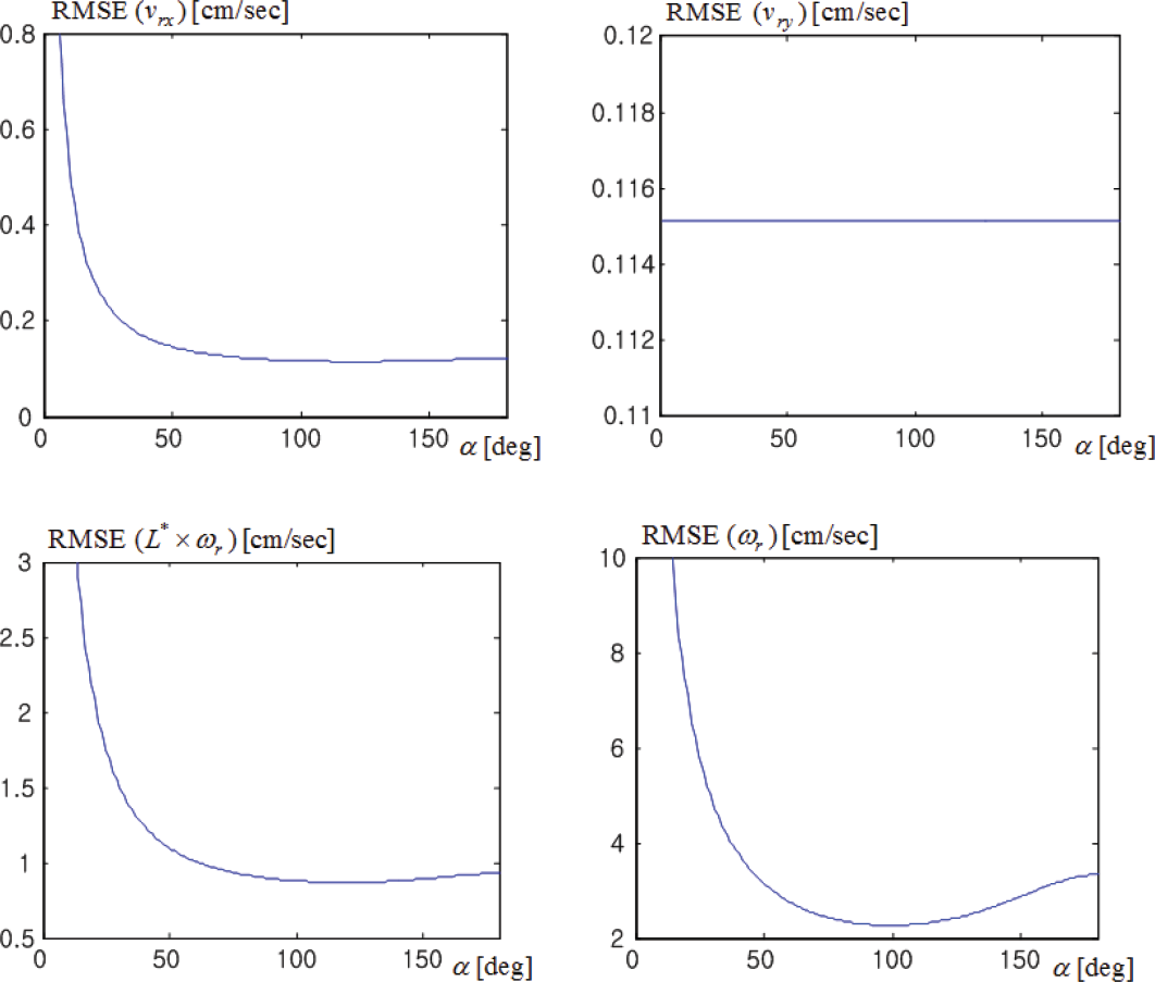
The changes of the root mean square errors of vrx, vry, L# × ω r , and ω r , according to the value of the angle α.
Now, assume that a mobile robot is commanded to rotate about the z axis at a velocity of vrx = vry = 0 cm/sec and ω
r
= 1 rad/sec (= 57.3 deg/sec). The same random noise vector
For the isotropic optical mouse placement Π1, Figure 10 shows the velocity measurements of the first optical mouse, and the resulting least squares velocity estimation of a mobile robot. Seen from Figure 10(a), the plots of v1x and v1y are noisy sinusoids, with the same amplitude of ρ
i
= b(= 16cm) but there is a phase difference of 90° between them; the plots of v2x and v2y are also noisy sinusoids, with the same amplitude of

In the case of the isotropic optical mouse placement Π1, the least squares estimation for an angular velocity of a mobile robot: (a) the measured velocity components, v1x, v1y, v
2x
and v2y, and (b) the estimated velocity components,
For four optical mouse placements, Π1, Π2, Π3, and Π4, Table 3 lists the root mean square errors of four components of the estimated mobile robot velocity, denoted by
The root mean square errors of the measured and estimated velocity components

Finally, let us assume that a mobile robot is commanded to move forward and rotate at the same time, at a velocity of vrx = 0 cm/sec, vry = 20 cm/sec and ω
r
= 1 rad/sec (= 57.3 deg/sec). Again, the same random noise vector

In the case of the isotropic optical mouse placement Π1, the least squares estimation for a hybrid velocity of a mobile robot: (a) the measured velocity components, v1x, v1y, v2x and v2y, and (b) the estimated velocity components,
In practice, inaccurate optical mouse readings may occur in abnormal situations, typically caused by a sudden change in floor condition or excessive height above the floor [15]. Two representative methods have been proposed to detect the occurrence of abnormal situations and to reduce their effects on mobile robot velocity estimation. First, in [3] and [5], the violation of the kinematic constraint of a pair of optical mice was used to determine the correctness of optical mouse measurements. Second, in [4] and [16], the inconformity of each optical mouse to the consensus reached by all optical mice involved or a pair of optical mice was used to evaluate the reliability of optical mouse measurements. Note that [4] is our previous work. In both methods, the most inaccurate optical mouse measurement is selected and removed from new mobile robot velocity estimation or localization. Furthermore, the ICP (Iterative Closest Point) based localization method was proposed in [14], which is robust to inaccurate optical mouse readings.
In the mobile robot velocity estimation using optical mice, it is essential to maintain a constant height of the optical mice and the floor, as much as possible. As the height increases, the area covered by the camera increases, so that the ratio of the relative displacement counts per real world length is subject to change [15]. To maintain a constant height from the floor, spring mechanisms were suggested to press optical mice to the floor [14, 16]. In [16], two leg springs are placed between a mobile robot and each of the four optical mice, in which small bumps on the floor possibly act as an obstacle to a mobile robot. In [14], two leg springs are placed between a mobile robot and a long arc-bended supporting plate with both of its ends connected to two optical mice by a rotating hinge. It seems that this mechanism can allow optical mice to traverse small bulges and also avoid excessive friction from the floor causing wheel slips [1].
Similar to this paper, the symbolic analysis of the Jacobian matrix and the optimal placement of optical mice were dealt with by Cimino and Pagilla [6]. However, there are two distinctive differences between the two works. First, the symbolic analysis of the Jacobian matrix, in this paper, provides the concise expressions of the eigenvalues, λ1 and λ3, in terms of Cx, Cy, and R, each of which has a clear geometrical meaning. With these concise expressions, which are in contrast to the complicated expressions in [6], the geometrical interpretations of both isotropic and singular optical mouse placements can be made, and also the condition for the anisotropic optical mouse placement with maximal isotropy can be readily derived. Second, both works deal with the same problem of optical mouse placement with a different criterion, with possible restrictions on the installation positions of optical mice at the bottom of a mobile robot. In contrast to [6], however, this paper can determine the optimal optical mouse placement, without any assumptions regarding the positions of optical mice.
Conclusion
In this paper, we presented the isotropy analysis and optimal placement of optical mice for mobile robot velocity estimation. Positional restrictions on the installation of optical mice at the bottom of a mobile robot were assumed. The main contributions of this paper include 1) the symbolic analysis of the Jacobian matrix, tailored to the isotropy analysis of the optical mouse placement, 2) the identification of the isotropic, anisotropic and singular optical mouse placements along with the corresponding characteristic lengths, and 3) the elaboration of the least squares mobile robot velocity estimation for the isotropic optical mouse placement. The results of this paper can be helpful especially for the development of personal robot mobile platforms with a non-circular base.
Footnotes
11.
This research was supported by Basic Science Research Program through the National Research Foundation of Korea (NRF) funded by the Ministry of Education (NRF-2012R1A1A2002175).