
Abstract
Detection and tracking strategies based on monocular vision are proposed for autonomous aerial refuelling tasks. The drogue attached to the fuel tanker aircraft has two important features. The grey values of the drogue's inner part are different from the external umbrella ribs, as shown in the image. The shape of the drogue's inner dark part is nearly circular. According to crucial prior knowledge, the rough and fine positioning algorithms are designed to detect the drogue. Particle filter based on the drogue's shape is proposed to track the drogue. A strategy to switch between detection and tracking is proposed to improve the robustness of the algorithms. The inner dark part of the drogue is segmented precisely in the detecting and tracking process and the segmented circular part can be used to measure its spatial position. The experimental results show that the proposed method has good performance in real-time and satisfied robustness and positioning accuracy.
1. Introduction
Aerial refuelling, also referred to as in-flight refuelling (IFR) or air-to-air refuelling (AAR), is an operation whereby fuel is transferred from one aircraft (the tanker) to another aircraft (the receiver) during flight. IFR is an important method for extending the flying distance and speed of the aircraft and is widely used in military aircraft. In unmanned aerial vehicles (UAV), autonomous air-to-air refuelling is needed to ensure flight endurance. There are two kinds of hardware configurations used for aerial refuelling: the first configuration, called the boom-and-receptacle refuelling system, includes a rigid boom extending from the tanker aircraft, with a probe and nozzle at its distal end. The boom also includes airfoils controlled by a boom operator stationed on the refuelling aircraft. The airfoils allow the boom operator to actively manoeuvre the boom with respect to the receiver aircraft, which flies in a fixed refuelling position below and aft of the tanker aircraft [1–5]. The second configuration, called the probe-and-drogue refuelling system, includes a refuelling hose which has a drogue deposited at its end trailed behind the tanker aircraft and a probe installed on the receiver aircraft. The probe must be placed or docked into the drogue in order to refuel successfully [6–9]. Autonomous aerial refuelling relies on three key technologies: target detection, tracking and measurement, in order to allow the receiver aircraft to determine control strategies to enable a robust and safe approach and coupling. The attempt described in this paper is to provide detection and tracking strategies for the probe-drogue autonomous aerial refuelling based on monocular vision.
In this paper, the drogue's detection and tracking strategies based on monocular vision are proposed for autonomous aerial refuelling tasks. Two important features of the drogue are used to design the detection and tracking strategies. The first feature is that the grey values of the drogue's inner part are almost the same and are different from the external umbrella ribs. The second feature is that the shape of the drogue's inner dark part is nearly circular. The drogue's detection algorithm includes two parts: the drogue's rough location algorithm and the drogue's fine positioning algorithm. The rough location algorithm is used to define the potential regions in which the drogue may be located, while the drogue's fine positioning algorithm is used to find the drogue in the potential regions accurately if the drogue is in the image. Particle filter is widely used in target tracking because of its robustness [10–13]. A new particle filter algorithm based on the drogue's shape was proposed to track the drogue. In the new particle algorithm, unique principles of state transition are defined to ensure tracking robustness even when the drogue's position or size changes significantly in two adjacent frames. A switch strategy between detection and tracking was proposed to improve the algorithm's robustness, which provides the link between detection and tracking. This is critical when the tracking has failed or the drogue is not in the image.
The paper is organized as follows. Section 2 gives an introduction to previous works. Section 3 describes the drogue's detection strategy. Section 4 describes the drogue's tracking strategy. Section 5 describes the switch strategy between detection and tracking. Section 6 presents the experimental results and Section 7 concludes the main points of the research.
2. Previous Works
Machine vision methods used for autonomous aerial refuelling tasks are becoming increasingly popular [6,7,14–17]. Advantages of using machine vision methods for autonomous aerial refuelling tasks include the potential for installation without modification being required to the target aircraft and increased measurement precision.
The researchers have developed a variety of different machine vision method for the probe-drogue autonomous aerial refuelling system (shown in Figure 1). John Valasek et al. [6] developed a vision-based navigation sensor and system for autonomous aerial refuelling tasks. For application to the endgame docking problem of automated aerial refuelling of aircraft, a VisNav sensor (a position-sensing diode) was mounted on a receiver aircraft and a set of LED beacons were mounted on a drogue being trailed from a tanker aircraft. When light energy from an individual beacon on the drogue was focused on the surface of the position-sensing diode, it generated an electrical current, which was measured with four pickoff leads, one on each side. The six-degrees-of-freedom position and attitude of the sensor aircraft with respect to the drogue can be computed by the four position-sensing signals. The main disadvantage of the method proposed in [6] is that some modifications to the tanker equipment must be made to provide electrical power for beacons, since there is no such power in the hose to which the drogue is attached. Fravolini et al. [18] proposed a docking control scheme for autonomous aerial refuelling of UAVs using a probe-drogue refuelling system. The docking control scheme was based on a fuzzy sensor fusion strategy featuring GPS and machine vision data. The GPS was used to measure the relative position between the tanker and the receiver and the machine vision was used to measure the relative camera-drogue distance. Some markers were placed in the drogue to measure its position and orientation. However, GPS receivers may be affected by interference from electronic devices and GPS signals may be blocked by the tanker. Lorenzo Pollini et al. [19] placed light emitting diodes (LEDs) on the drogue and used a CCD webcam with an infra-red filter to identify the LEDs. Hager and Mjolsness's (LHM) algorithm [20] was used to determine iteratively the translation vector as well as the transformation matrix between the 3D reference systems on the object and the camera, respectively. As in [6], the main disadvantage in [19] is that some modifications to the tanker equipment are required. Carol Martinez et al. [7] proposed a vision-based strategy for autonomous aerial refuelling tasks. The proposed strategy consisted of four stages: detection, initialization, tracking and 3D position estimation. The detection stage was composed of two algorithms: one based on edge-image template matching using the normalized cross correlation (NCC) method, and the second based on image threshold segmentation. The detection method is time-consuming because the drogue images with different variations, such as scale, illumination and position, must be contained in the template images. It is impossible to contain all the conditions of the drogue in the template images, so in order to decrease the failure of detection, an experience threshold was used to segment the image to detect the inner part of the drogue when the edge-image template matching method failed. However, the experience threshold is hard to define because the illumination of the scene may change significantly. The tracking algorithm was a Hierarchical Multi-Parametric and Multi-Resolution implementation of the Inverse Compositional Image Alignment technique HMPMR-ICIA [21].

The probe-and-drogue refuelling system
3. Detection Strategy
3.1. Rough Location of the Drogue
The aim of rough location is to define the potential regions in which the drogue may be located. According to prior knowledge, the rough location stage is composed of two algorithms: this first based on image segmentation using a series of thresholds, and the second based on contour features of the image regions segmented by image segmentation using a series of thresholds.
It is impossible to define an accurate experience threshold used to segment the image to detect the inner part of the drogue because the illumination of the scene may change significantly. So a series of thresholds are used to segment the same image, as follows:


where f is the input images, F is the set of output images which include {g T0 , g T1 ,…, gTN-1}. {T 0 , T 1 ,…, TN-1} are a series of thresholds used to segment the input image, as follows:

where ∆T is an increment of the threshold.
Then all the contours of the output images are extracted, and the set of the contours is expressed as C = {c 0 , c 1 ,…, c n-1 }. The contour of the inner part of the drogue is nearly circular, so aspect ratios of the minimum enclosing rectangles of contours are used to define the potential contours of the drogue from the set C, as follows:
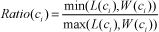


where Ratio(c
i
) is the aspect ratios of the minimum enclosing rectangle of the contour and T
Ratio
is threshold of the aspect ratios of the minimum enclosing rectangle. L(c
i
) is the length of the minimum enclosing rectangle, T
L1
is the lower bound of the length of the minimum enclosing rectangle and T
L2
is the upper bound of the length of the minimum enclosing rectangle. W(c
i
) is the width of the minimum enclosing rectangle, T
W1
is the lower bound of the width of the minimum enclosing rectangle and T
W2
is the upper bound of the width of the minimum enclosing rectangle.
In order to improve the speed of detection, the Multi-Resolution (MR) hierarchical structure [22] is used. The MR structure is created by repeatedly downsampling the images by a factor of two in order to create the different levels of the pyramid. The number of levels pL is defined, taking into account the size of the drogue in the image. The general idea of the acceleration strategy is that the rough location of the drogue is conducted at the lowest resolution level. The advantage of using the MR structure is that many small error contours will not be segmented out at low resolutions.
3.2. Fine Positioning of the Drogue
3.2.1. Location of Edge Points of the Drogue's Inner Dark Part
To every contour in the set of


where (c
i
centX
, c
i
centY
) are the coordinates of the centre of the contour
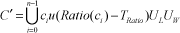
where T
d
is a threshold for eliminating unnecessary contours,
In order to obtain the location of edge points of the drogue's inner dark part, some half-lines are assumed to start at the point (

where p is the point in the half-line k,
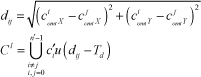
Most of directions of the half-lines are neither horizontal nor vertical, so coordinate transformations are used to calculate the coordinates of small rectangles in half-lines whose directions are not horizontal or vertical. Figure 3 shows three coordinate systems; the coordinate system (X 0 , Y 0 ) is centred on the upper-left corner of the image, the X 0 axis points to the right horizontally and the Y 0 axis points vertically downwards. The coordinate system (X 1 , Y 1 ) is centred at the point (x 1 , y 1 ) which is the translation relative to the point O 0 . The X 1 axis is parallel to the X 0 axis and the Y 1 axis is parallel to the Y 0 axis, but their directions are opposite. The coordinate system (X 2 , Y 2 ) is centred at the point (x 1 , y 1 ). The X 2 axis overlaps with the half-line i and the Y 2 axis is perpendicular to the X 2 axis.

Location of edge points of the drogue's inner dark part
Three coordinate systems
The coordinates of the point A are (a 0 , b 0 ) in the coordinate system (X 0 , Y 0 ), (a 1 , b 1 ) in the coordinate system (X 1 , Y 1 ) and (a 2 , b 2 ) in the coordinate system (X 2 , Y 2 ). The relationship between (a 1 , b 1 ) and (a 2 , b 2 ) is:

and the relationship between (a 0 , b 0 ) and (a 1 , b 1 ) is:

From (14) and (15), the relationship between (a 0 , b 0 ) and (a 2 , b 2 ) can be obtained as follows:

The parameter θ is the angle between the X 1 axis and the X 2 axis. The coordinates of points in the coordinate system (X 0 , Y 0 ) can be calculated by equation (16) if the coordinates in the coordinate system (X 2 , Y 2 ) are known in advance.
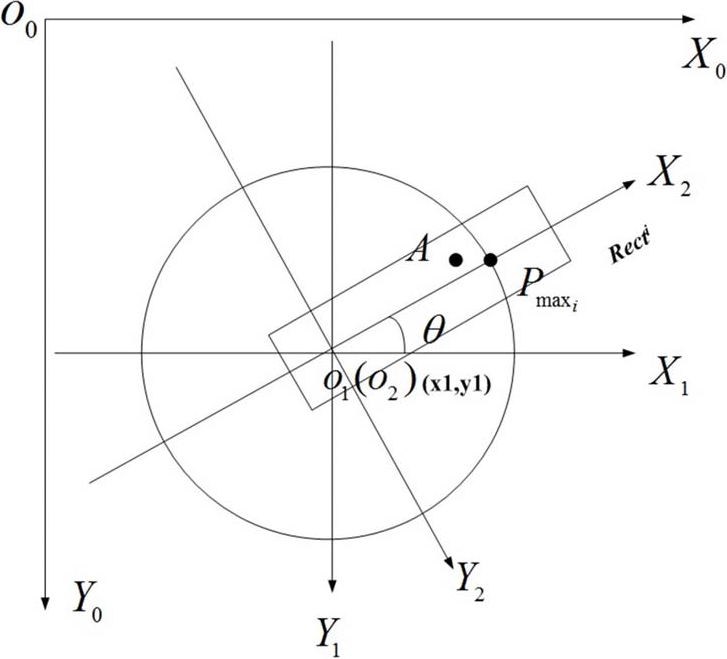
In order to improve the computing speed, the integral image is used to calculate the ratio of the small rectangle's two parts. The Rect i in Figure 3 and Figure 4 is the rectangle that is used to calculate the integral image in the half-line i. The height of the rectangle Rect i is the same as the heights of the small rectangles which move along the half-lines in Figure 2: all are H. The widths of the small rectangles are W and the width of the rectangle Rect i is W+N s . N s is the moving time of the small rectangle in every half-line. The integral image of the rectangle Rect i is calculated as follows:

The rectangle Rect i used to calculate the integral image

where s(y) is the sum of the y-th column pixels, ii(H, y) is the value of the last line of the integral image. In Figure 4, l1 is the boundary of the small rectangle's two parts, l2 is the left side of the small rectangle and l3 is the right side of the small rectangle. The value of the integral image at location 2 is the sum of the pixels in rectangle A. The value of the integral image at location 1 are the sum of the pixels in rectangle A+B and the value of the integral image at location 3 is the sum of the pixels in rectangle A+B+C. Therefore, the sum of the pixels in rectangle B is ii1- ii2 and the sum of the pixels in rectangle C is ii3- ii1. The ratio of the small rectangle's two parts is (ii3- ii1)/ (ii1- ii2), while ii1, ii2, ii3 are the values of the integral image at locations 1, 2 and 3 respectively.
3.2.2. Getting Rid of the Bad Edge Points Using Vector Angles
The bad edge points of the drogue's inner dark part may be detected because of image noise or the partial occlusion of the drogue. Assume that the detected edge points of the drogue's inner dark part are the red points {1, 2,…, 16} shown in Figure 5. We define the vectors as {

Vector angles of edge points

where P={p0, p1,…, pn1} is the set of the remaining edge points after getting rid of the bad edge points using vector angles, n p is the number of the edge points detected in Section 3.2.1, n1 is the number of the remaining edge points after getting rid of the bad edge points using vector angles, θ T is the threshold of the vector angles, θ i is the vector angle of the edge point and the function u(t) is defined in (9). The bad edge points 4, 8, 13 and 15 in Figure 5 can be eliminated by equation (18).
3.2.3. Location of the Drogue Using RANSAC
The styles of the bad edge points are diverse, so some bad edge points cannot be eliminated by vector angles. For example, the bad point 9 in Figure 5 cannot be eliminated by the vector angle because the vector angle θ9 is less than the threshold θ
T
of the vector angles. The shape of the drogue's inner dark part is nearly circular, so good edge points can be determined by this prior knowledge. RANSAC [24], an abbreviation for “random sample consensus”, is an iterative method to estimate parameters of a mathematical model from a set of observed data which contains outliers. Each contour

A threshold T
W
is used to define whether the set
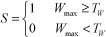
where S is the state of detection, S=1 indicates there is a drogue in the image and S=0 indicates there isn't a drogue in the image. The pseudo-code of the algorithm for location of the drogue using RANSAC is presented in Figure 6.

Location of the drogue using RANSAC
4. Tracking Strategy
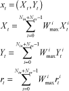
The tracking algorithm is based on particle filters which are sequential Monte Carlo methods [25] based on point mass. Particle filters are suitable for any non-linear system that could be represented by a state model. The tracking object is the inner dark part of the drogue in the tracking algorithm, so the centre of the inner dark part of the drogue can be defined as the state x t of the drogue at time t.
4.1. Selection of Particles and State Transition
The disturbance of the drogue is uncertain when in the air, so it is hard to establish the accurate motion model of the drogue during air-to-air refuelling. The state xt-1 of the drogue at time t-1 is selected as the particle at time t. The number of the particle is N
in
+ N
ex
. N
in
is the number of particles called interior particles whose range of state transition is limited to the interior of the circle C
cir
whose centre is xt-1 and radius is r, while N
ex
is the number of particles called exterior particles whose range of state transition is limited to some half-lines in the exterior of the circle C
cir
. In Figure 7, the half-lines to which exterior particles whose range of state transition is limited are assumed to start at the position which is l away from the centre xt-1, and extend outward. The angle between two adjacent half-lines is θ and the distance between two adjacent exterior state transition particles in the same half-line is
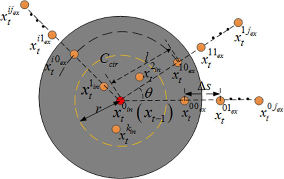
Principles of state transition.
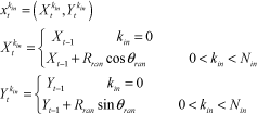
where

where
4.2. Particle weights and posterior probability
The particle weights of state transition particles in Section 4.1 can be calculated through the following steps:
Obtain the set
Eliminate the bad edge points of every set
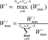
Calculate weights of state transition particles using the RANSAC method with the same method in Section 3.2.3, and the weight of jth state transition particle can be expressed as W j max .
A threshold T
P
is used to get rid of bad state transition particles as follows:

Calculate the state weight at time t and normalize the weights of state transition particles as follows:
5. Switch Strategy between Detection and Tracking
The detection stage must be enabled automatically to detect the drogue either at the start of the run or when the drogue has gone out of the field of view of the camera, or alternatively because the tracking algorithm has failed to track the drogue. Therefore, performance assessment criteria should be defined to switch between detection algorithm and tracking algorithm. The detection and tracking algorithm is initiated with a lost status L=1(i.e.. no drogue has been detected). The detection algorithm is then enabled to find the drogue. The drogue is detected successfully when the state of detection S=1 in Section 3.2.3, then the lost status is L=0 and the tracking algorithm is enabled. The performance assessment criteria of the tracking algorithm can be defined according to the weights of the drogue's states in k s successive frames as follows:

where δ(t) is defined in (3), u(t) is defined in (9), W i is the state weight at time I and T t is a fixed threshold. If the lost status is L=0, the tracking algorithm continues running. If the lost status is L=1, the tracking algorithm is stopped and the detection stage is enabled in the region of interest (ROI) of the image. The lost status is L=0 and the tracking algorithm is enabled if the drogue is detected successfully, otherwise the lost status is L=1 and the detection stage is enabled in all regions of the image. The process of the strategy for switching between detection and tracking is shown in the proposed visual detecting and tracking system for air-to-air refuelling in Figure 8.

The proposed visual detecting and tracking system for air-to-air refuelling
6. Experimental Results
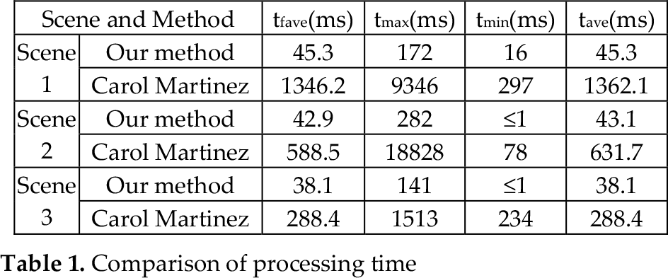
In this section, experiments were conducted on the real drogue of air-to-air refuelling at different air scenes. The performance of our method was compared to the performance of the algorithm proposed by Carol Martinez et al. [7]. Three experiments were carried out to detect and track different drogues at different air scenes. Speed of processing and percentage of correct location are compared between Carol Martinez's method and ours. The speed indicators were the average time t fave of processing each image, the maximum time t max , the minimum time t min and the average time t ave between the adjacent outputs when the drogue was in the image. The percentages of correct location are compared between Carol Martinez's method and ours at different location error thresholds. The proposed algorithm was developed in C++ and the OpenCV libraries were used for managing image data and the experiments were carried out on a PC with a AMD Athlon (tm) II X4 645 Processor and a 3.1GH clock.
6.1. At Air Scene 1
125 frames of images with 1440×900 pixel size were used in the experiment at air scene 1. The experimental data were obtained from the website http://www.youtube.com/watch?v=nWmFpLVl8MQ. Eleven edge templates as shown in Figure 9 were used to find the drogue in the lowest resolution image in the image pyramid, the number of pyramid levels was pL=3 and the threshold used to segment the image was 85 in Carol Martinez's method [7]. In our method, the number of pyramid levels in the application was pL=3, the lowest threshold was T 0 =20, the number of thresholds was k=53 and the increment of the threshold was ΔT=3 in equation (4), The aspect ratio was T Ratio =0.7, the lower bound of the length of the minimum enclosing rectangle was T L1 =4 and the upper bound of the length of the minimum enclosing rectangle T L2 was equal to one third of the image's height in (6). The lower bound of the width of the minimum enclosing rectangle was T W1 =4 and the upper bound of the width of the minimum enclosing rectangle T W2 was equal to one third of the image's width in (7) and (8). The threshold for eliminating unnecessary contours was T d =1.5 in (12); the number of the half-lines corresponding to each contour was 20, the length of each half-line was 60, the height of the small rectangle was three and the width of the small rectangle was eight in Section 3.2.1, The threshold of the vector angles was θ T =80° in (18); the threshold T W was 15 in (20); the number of samples was n s =5 and the threshold T r was six in the pseudo-code in Section 3.2.3, The number of interior particles was N in =20, the number of exterior particles was N ex =45, the radius of the circle C cir was 15 and the parameter l was 15. The distance between two adjacent exterior state transition particles in the same half-line was Δs=22. Three exterior particles were in the same half-line and the angle between two adjacent half-lines was θ=24° in 4.1. The threshold T P was 15 in 4.2; the threshold T t was 15 in Section 5.
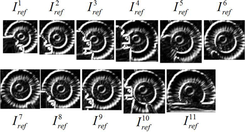
Edge templates at air scene 1 in the method of Carol Martinez et al
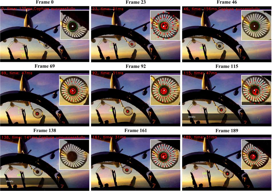
Nine result frames in our method are shown in Figure 10. The magnified target is displayed in the top-right corner of the frame in Figure 10. The green circle segmented in detecting and tracking process is the inner dark part of the drogue, the white point is the green circle's centre and the red points are the state transition particles in Figure 10. The comparison of processing time of each frame between our method and the method of Carol Martinez et al. is shown in Figure 11. The processing time of each frame in our method is clearly less than the processing time in the method of Carol Martinez et al. The processing time in our method is not affected by the scale of the drogue in the image. In Figure 11, the cyan triangle is the detection time (about 16ms) in ROI in the 116th frame and the nine magenta pentagrams stand for the detection time (less than 172ms) in the whole images in our method. The green squares represent the time in which no data is output (or the algorithm thinks there is no target in the frame) in Carol Martinez's method. As shown in Figure 11, no data is output from the 32th frame to the 39th frame, though the targets in these frames are clear in Carol Martinez's method, while our method gives the drogue's positions in the entire frames. In the method of Carol Martinez et al., the processing time is affected by the size of the reference image. The detecting algorithm finds the first reference image with pixel size 213×206 in the 0th frame as shown in Figure 11 and the average tracking time corresponding to the first reference image is 1099.5ms. The detecting algorithm finds the second reference image with pixel size 217×213 in the fifth frame as shown in Figure 11 and the average tracking time corresponding to the second reference image is 1163.3ms. The detecting algorithm finds the third reference image with pixel size 246×254 in the 40th frame as shown in Figure 11 and the average tracking time corresponding to the second reference image is 1555.4ms. The speed indicators in our method are better than the method of Carol Martinez et al. as shown in Table 1. The percentage of correct location in the method of Carol Martinez et al. is less than 30%; in our method it is 100% when the location error threshold is five pixels, as shown in Figure 18.

Nine result frames at air scene 1 in our method
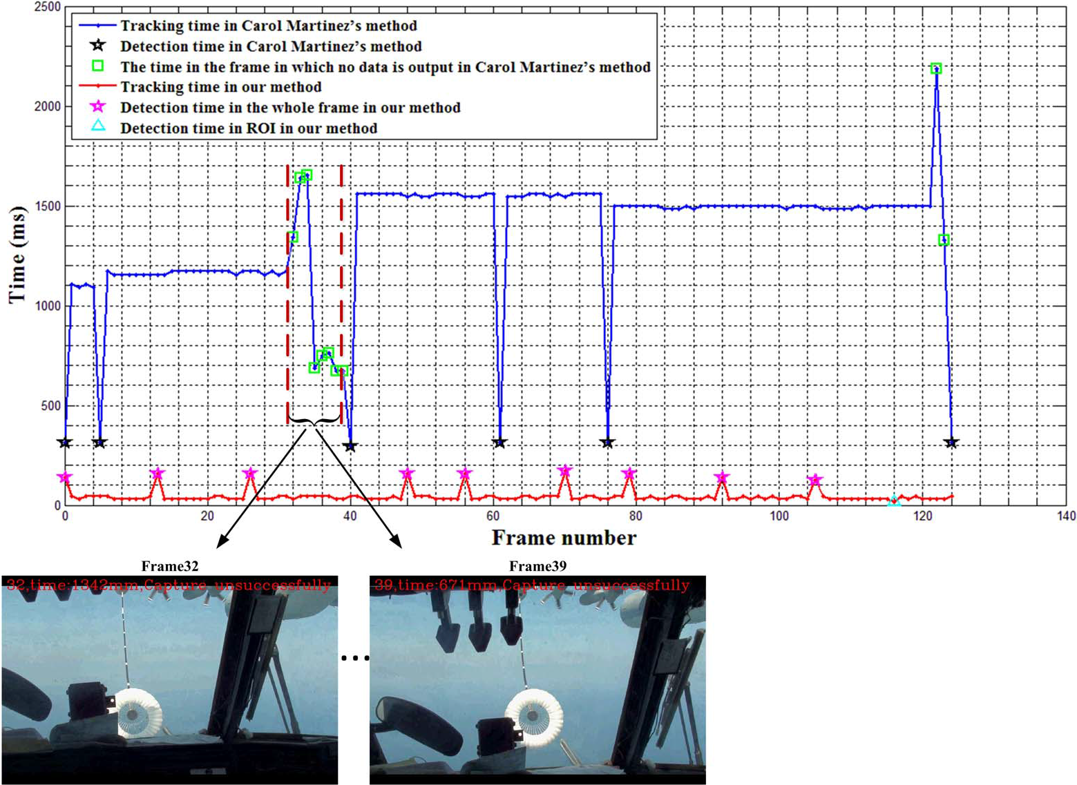
The processing time at the air scene 1
Comparison of processing time
6.2. At Air Scene 2
One hundred and ninety frames of images with pixel size 1440×900 were used in the experiment at air scene 2. The experimental data were obtained from the website http://www.youtube.com/watch?v=cG6rMZF6mIw. The appearance of the drogue at air scene 2 was different from the appearance of the drogue at air scene 1, but both had the two important features. Eleven edge templates were used to find the drogue as shown in Figure 12 and the threshold used to segment the image was 40 in Carol Martinez's method. The parameters in our method are the same as the parameters in Section 6.1. Nine result frames are shown in Figure 13 and the processing time of each frame is shown in Figure 14 in our method. The processing time of each frame in our method is clearly less than the processing time in the method of Carol Martinez et al. as shown in Figure 14.

Edge templates at air scene 2 in the method of Carol Martinez et al
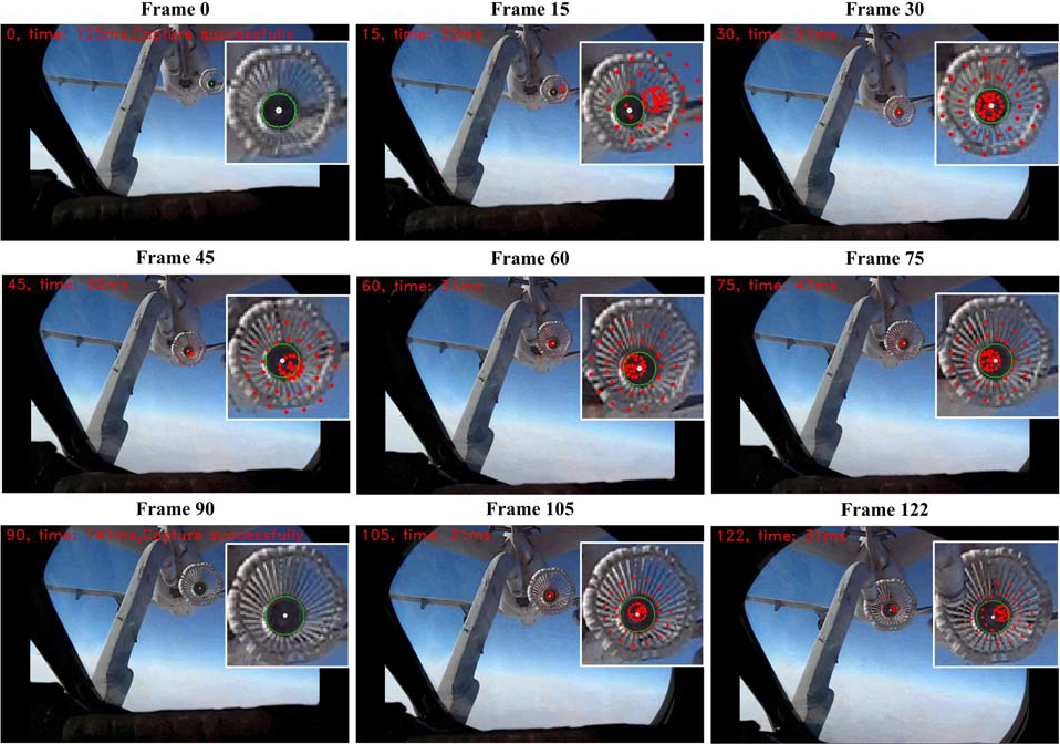
Nine result frames at air scene 2 in our method

The processing time at air scene 2
In Figure 14, the seven cyan triangles are the detection time in ROI and the 11 magenta pentagrams stand for the detection time in the whole frames in our method. The detection time represented as the black pentagrams in Figure 14 in Carol Martinez's method is obviously greater than the detection time in our method. The green squares are the time in which no data is output in Carol Martinez's method. As shown in Figure 14, no data is output from the 121th frame to the 129th frame and a wrong target is detected and tracked from the 130th frame to the 136th frame. This is probably because the drogue is partially occluded. In our method, only in the 138th frame is no danger output. The speed indicators in our method are better than the method of Carol Martinez et al., as shown in Table 1. The percentage of correct location in the method of Carol Martinez et al. is less than 20%, while in our method it is near 80% when the location error threshold is five pixels, as shown in Figure 18.
6.3. At Air Scene 3
123 frames of images with 1440×900 pixel size were used in the experiment at air scene 3. The experimental data were obtained from the website http://www.jokeroo.com/videos/cool/aerial-refueling.html.
The appearance of the drogue at air scene 3 was different from the appearance of the drogues at air scene 1 and air scene 2, but all of them had two important features. Eleven edge templates were used to find the drogue as shown in Figure 15 and the threshold used to segment the image was 50 in Carol Martinez's method. The parameters in our method are same to the parameters in Section 6.1. Nine result frames are shown in Figure 16 and the processing time of each frame in our method is shown in Figure 17. The processing time of each frame in our method is clearly less than the processing time in the method of Carol Martinez et al. as shown in Figure 17 since the HMPMR-ICIA [21] algorithm adopted by Carol Martinez is a time-consuming iterative optimization method during tracking. The speed indicators in our method are better than the method of Carol Martinez et al., as shown in Table 1. The percentage of correct location in the method of Carol Martinez et al. is less than 70%, while in our method it is more than 80% when location error threshold is five pixels, as shown in Figure 18.

Edge templates at air scene 3 in the method of Carol Martinez et al
Nine result frames at air scene 3 in our method

The processing time of each frame at air scene 3

Percentages of correct location at different location error thresholds
7. Conclusions
Detecting and tracking strategies for aerial refuelling tasks based on monocular vision were proposed. According to the drogue's prior knowledge, multi-threshold segmentation and shape-distinguishing arithmetic were used to detect the drogue. Multi-threshold segmentation decreased the rate of missed detection and the figure=distinguishing arithmetic pinpointed the drogue's position precisely. A new particle filter algorithm based on the drogue's shape was proposed to track the drogue. In the new particle algorithm, unique principles of state transition are defined to ensure tracking robustness even when the drogue's position or size change significantly in two adjacent frames. A strategy of switching between detection and tracking was proposed and the switching strategy enhanced robustness of our method. In the method, the inner dark part of the drogue was segmented precisely in the detecting and tracking process and the segmented circular part can be used to measure the spatial position of the drogue. The speed of the proposed method is fast, is less affected by the size of the drogue in the image and it is highly accurate. In the future, we will try to use the segmented circular part to measure the position of the drogue in Cartesian space based on monocular vision by the method of combing the 3D model of the drogue and the imaging principle.
Footnotes
8. Acknowledgments
This work is partly supported by National Natural Science Foundation of China under Grant 61227804 and 61105036.