Forward and Inverse Dynamics of the Biped PASIBOT

Abstract

This article addresses the supporting foot slippage of the biped robot PASIBOT and develops its forward and inverse dynamics for simple and double support phases. To address the slippage phenomenon, we consider an additional degree of freedom at the supporting foot and also distinguish between static and kinetic friction conditions. The inverse and forward dynamics, accounting for support foot slippage, are encoded in MATLAB. The algorithm predicts the motion of the biped from the torque function given by the biped's sole motor. Thus, the algorithm becomes an indispensable tool for studying transient states of the biped (for example, the torques required for starting and braking), as well as defining the conditions that prevent or control slippage. Since the developed code is parametric, its output can greatly assist in the design, optimization and control of PASIBOT and similar biped robots. The topology, kinematics and inverse dynamics of the one-degree-of-freedom biped PASIBOT have been previously described, but without regard to slippage between the supporting foot and the ground.

1. Introduction

The development of humanoid robots, particularly bipedal walking robots, is of major interest in robotics. As a result, a wide variety of refined designs have been proposed. The introduction of new mechanisms and kinematic chains has enabled walking robot designs with fewer actuators and gearboxes, thereby reducing the weight, power consumption and cost of operation without compromising walking functionality [1, 2].

Most of the proposed solutions are based on the human leg, in which the links (femurs, tibias and feet) are connected by joints (hip, knee and ankle), all or most of which are operated in the robots by actuators (such as motors, pneumatic devices and artificial muscles) [3]. Alternatively, researchers aim to emulate the walking motion by combining various classical mechanisms. Ceccarelli and his team, working from the latter perspective at the Laboratory of Robotics and Mechatronics (LARM), have presented the biped robot EP-WaR II [4]. More recently, the group have developed the low-cost humanoid legs CALUMA [5] and have begun work on other designs [6].

The MAQLAB group at Universidad Carlos III in Madrid, from the same perspective, have designed and manufactured the biped PASIBOT [1, 2].

The aims of analysing the mechanical performance of bipeds are twofold: to develop increasingly complex and powerful robots and to increase efficiency and autonomy [7]. As an example of the latter, the external forces and inertias acting on passive and quasi-passive bipeds are manipulated to minimize the power loss [8, 9].

Biped locomotion has been studied from several perspectives. Much effort has been devoted to the design of optimal trajectories and stabilized walking cycles via control programs. However, the slippage problem has been largely ignored. Moreover, an assumption of standard control strategies is that the contact point with the walking surface is static along the walking axis.

Little work has been devoted to the kinematics and dynamics of the slip of the supporting contact. To incorporate these effects requires new equations and additional degrees of freedom, as implemented in [10, 11].

The kinematics of PASIBOT is detailed in [1]. In that study, a program based on inverse dynamics calculates the torque required in the sole motor for PASIBOT to walk steadily with a non-sliding supporting foot. This parametric code proved useful in the recursive design of the biped, as illustrated in [12]: minimizing the torque of the motor minimizes its weight and hence the weight of the links of the biped, permitting a lighter engine [13]. This cyclical design process becomes complicated when biped transients such as starting and stopping, and sliding of the supporting foot, are included.

In this article, we present a parametric program that solves the forward dynamics of the biped. The program accepts the initial kinematic state and the motor torque (as a function of time) as inputs, and returns the bipedal movement, including sliding of the supporting foot in both single and double support phases. The sliding is taken into account by adding one degree of freedom. Thus, we focus on the kinematics and dynamics of the sliding supporting foot.

2. Biped robot prototype

PASIBOT is a one-degree-of-freedom mechanical system based on a combination of classical mechanisms that emulates human walking to some extent (at least regarding the trajectories of the knees and feet). A prototype of PASIBOT, modelled with the solid modelling software Solid Edge (Siemens PLM, USA), is shown in Fig. 1.

Figure 1.

Prototype of PASIBOT, built by the MAQLAB research group at Universidad Carlos III, Madrid

In Fig. 2, all links belonging to the supporting leg are named and numbered as in [1]. Corresponding links of the swinging leg are identified by primes.

Figure 2.

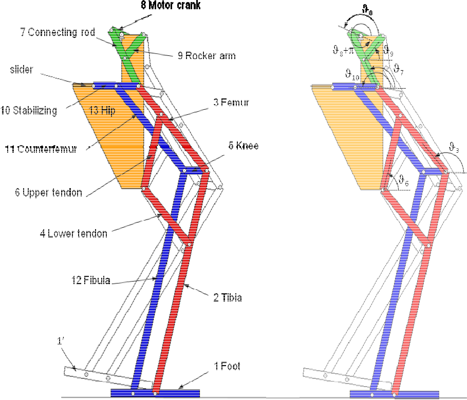
Links of PASIBOT: Left: nomenclature and numeration of the supporting leg. Right: angles for the links of the supporting leg; the links of the swinging leg are identified by primes.

The coordinates describing the position of link i are the angle ϑi and the centre of mass Cartesian coordinates xi and yi.

In this article, when the supporting foot is considered fixed, the horizontal centre of mass coordinate of link i is denoted by Xi, whereas xi implies that slippage of the supporting foot is allowed.

3. Kinematic analysis of pasibot allowing for sliding of supporting foot

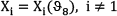
In the preliminary kinematic analysis of PASIBOT [1], a fixed supporting foot was assumed, so the biped possessed a single degree of freedom (DOF). Thus, the angular positions and the Cartesian coordinates of the centre of mass of link i are referred to the angular position of the motor crank (ϑ8):

${\mathrm{\vartheta }}_{\mathrm{i}}={\mathrm{\vartheta }}_{\mathrm{i}}\left({\mathrm{\vartheta }}_8\right),\mathrm{\hspace{0.17em}}\mathrm{i}=\mathrm{2,3}...1\mathrm{\text{'}},2\mathrm{\text{'}},...\left(\mathrm{i}\ne 8\right)$

(1)

${\mathrm{X}}_{\mathrm{i}}={\mathrm{X}}_{\mathrm{i}}\left({\mathrm{\vartheta }}_8\right),\mathrm{\hspace{0.17em}}\mathrm{i}\ne 1$

(2)

${\mathrm{y}}_{\mathrm{i}}={\mathrm{y}}_{\mathrm{i}}\left({\mathrm{\vartheta }}_8\right),\mathrm{\hspace{0.17em}}\mathrm{i}\ne 1$

(3)

In Eq. (2), Xi denotes a no-slip condition of the supporting foot, as distinct from the case in which the supporting foot is allowed to slip (see Eq. 4). Such a distinction is not necessary for ϑi and yi, because both variables are independent of supporting foot slippage. Moreover, note that all coordinates are relative to the fixed supporting foot (i = 1), and hence ϑ1 =0; X1 =0; y1 = 0.

However, if any slippage between the supporting foot and the floor is allowed, the biped becomes a 2-DOF mechanism (note that the robot moves across a plane, and the supporting foot supposedly remains horizontal). Now, let the x-coordinate of the foot, x1, be an additional independent coordinate. Eqs. (1) and (3) remain valid for the angular coordinate and the vertical centre of mass coordinate, respectively, of link i, while the horizontal centre of mass coordinate increases by the value of the supporting foot slippage x1 as follows:

${\mathrm{x}}_{\mathrm{i}}={\mathrm{x}}_1\mathrm{\hspace{0.17em}}+\mathrm{\hspace{0.17em}}{\mathrm{X}}_{\mathrm{i}}\left({\mathrm{\vartheta }}_8\right);\mathrm{\hspace{0.17em}}\mathrm{i}\ne 1$

(4)

The first and second time derivatives of Eq. (4) are as follows:

$\begin{array}{l}\stackrel{.}{{\mathrm{x}}_{\mathrm{i}}}=\frac{\mathrm{d}{\mathrm{x}}_1}{\mathrm{d}\mathrm{t}}+\frac{\mathrm{d}{\mathrm{X}}_{\mathrm{i}}}{\mathrm{d}{\mathrm{\vartheta }}_8}\frac{\mathrm{d}{\mathrm{\vartheta }}_8}{\mathrm{d}\mathrm{t}}={\stackrel{.}{\mathrm{x}}}_1+{\mathrm{X}}_{\mathrm{i}}\mathrm{\prime }\left({\mathrm{\vartheta }}_8\right)\stackrel{.}{{\mathrm{\vartheta }}_8}\\ {\stackrel{..}{\mathrm{x}}}_{\mathrm{i}}={\stackrel{..}{\mathrm{x}}}_1+{\mathrm{X}}_{\mathrm{i}}\mathrm{\prime }\mathrm{\prime }\left({\mathrm{\vartheta }}_8\right){\stackrel{.}{{\mathrm{\vartheta }}_8}}^2+{\mathrm{X}}_{\mathrm{i}}\mathrm{\prime }\left({\mathrm{\vartheta }}_8\right){\stackrel{..}{\mathrm{\vartheta }}}_8\end{array}$

(4 bis)

where a prime denotes an explicit derivative with respect to ϑ8, and dots denote a time derivative.

4. Dynamics of Pasibot: Inverse Vs. forward dynamics – Fixed Vs. sliding supporting foot

The dynamics of mechanical systems can be modelled in two ways: inverse dynamics, which calculates the forces and torques that produce kinematics (movement); and forward dynamics, which computes the movement from known applied forces and torques.

In biped dynamics, we can also distinguish between a fixed and a sliding supporting foot.

As stated in [1], we applied inverse dynamics to parametrically calculate the required torque at the sole motor for PASIBOT to walk at a steady state (constant speed) with no sliding between the supporting foot and the floor. However, in the transitional regime, when sliding between the supported foot and the floor is allowed during starting or stopping, the kinematics is unknown and other dynamical approaches must be applied.

To study the resistance and deformations of every link, we require knowledge of the forces acting between the links. To this end, we employ a Newton–Euler dynamic scheme.

Following the nomenclature introduced in [1], the dynamics of link i is described as follows:

$\begin{array}{c}\left\{\begin{array}{l}\sum _{\mathrm{j}<i}{\mathrm{f}}_{{\mathrm{j}\mathrm{i}}_{\mathrm{x}}}-\sum _{\mathrm{k}>i}{\mathrm{f}}_{{\mathrm{i}\mathrm{k}}_{\mathrm{x}}}={\mathrm{m}}_{\mathrm{i}}{\stackrel{..}{\mathrm{x}}}_{\mathrm{i}}\\ \sum _{\mathrm{j}<i}{\mathrm{f}}_{{\mathrm{j}\mathrm{i}}_{\mathrm{y}}}-\sum _{\mathrm{k}>i}{\mathrm{f}}_{{\mathrm{i}\mathrm{k}}_{\mathrm{y}}}={\mathrm{m}}_{\mathrm{i}}\mathrm{g}+{\mathrm{m}}_{\mathrm{i}}{\stackrel{..}{\mathrm{y}}}_{\mathrm{i}}\\ \sum _{\mathrm{j}<i}{\mathrm{T}}_{\mathrm{j}\mathrm{i}}-\sum _{\mathrm{k}>i}{\mathrm{T}}_{\mathrm{i}\mathrm{k}}+\\ +\sum _{\mathrm{j}<i}\left({{\mathrm{r}}_{{\mathrm{i}\mathrm{j}}_{\mathrm{x}}}\mathrm{f}}_{{\mathrm{j}\mathrm{i}}_{\mathrm{y}}}-{{\mathrm{r}}_{{\mathrm{i}\mathrm{j}}_{\mathrm{y}}}\mathrm{f}}_{{\mathrm{j}\mathrm{i}}_{\mathrm{x}}}\right)-\sum _{\mathrm{k}>i}\left({{\mathrm{r}}_{{\mathrm{i}\mathrm{k}}_{\mathrm{x}}}\mathrm{f}}_{{\mathrm{i}\mathrm{k}}_{\mathrm{y}}}-{{\mathrm{r}}_{{\mathrm{i}\mathrm{k}}_{\mathrm{y}}}\mathrm{f}}_{{\mathrm{i}\mathrm{k}}_{\mathrm{x}}}\right)={\mathrm{I}}_{\mathrm{i}}{\stackrel{..}{\mathrm{\vartheta }}}_{\mathrm{i}}\end{array}\right.\\ \mathrm{i}\mathrm{\hspace{0.17em}}=\mathrm{\hspace{0.17em}}1,...,\mathrm{13,1}\mathrm{\text{'}},...,7\mathrm{\text{'}},9\mathrm{\text{'}},...,12\mathrm{\text{'}}\end{array}$

(5)

where Newton's third law has been used to reduce the number of unknown forces. Note that because links 8′ and 13′ do not exist, the biped contains 24 links, and hence Eq. (5) is a system of 24 × 3 = 72 equations. However, as explained below, the torque equation for the supporting foot is usually considered separately.

4.1. Inverse Dynamics and Fixed Supporting Foot

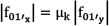
When dealing with inverse dynamics in the fixed supporting foot scenario (x1 = 0, xi = Xi), Eq. (5) reduces to a linear equation system in which the torques Tij and forces (fijx, fijy) are unknown. Revolute joints are assumed to be ideal, so that all torques between links are zero. That is, Tij = 0, except for the motor torque T13,8 = – T8,13 ≡ T8, between the hip and the crank. The forces between the floor and the supporting foot, f01x and f01y, are the friction and normal forces, respectively.

The system Eq. (5) is linear if the torque equation for the supporting foot (link 1; see Fig. 3) is excluded. The torque of the supporting foot is described by the following equation:

Figure 3.

Forces acting on the supporting foot (link 1). Link 1 is connected to links 2 and 12. The floor is considered as link 0.

$\begin{array}{c}{\mathrm{r}}_{{10}_{\mathrm{x}}}{\mathrm{f}}_{{01}_{\mathrm{y}}}-{\mathrm{r}}_{{10}_{\mathrm{y}}}{\mathrm{f}}_{{01}_{\mathrm{x}}}-\left({\mathrm{r}}_{{12}_{\mathrm{x}}}{\mathrm{f}}_{{12}_{\mathrm{y}}}-{\mathrm{r}}_{{12}_{\mathrm{y}}}{\mathrm{f}}_{{12}_{\mathrm{x}}}\right)-\\ -\left({\mathrm{r}}_{{\mathrm{1,12}}_{\mathrm{x}}}{\mathrm{f}}_{{\mathrm{1,12}}_{\mathrm{y}}}-{\mathrm{r}}_{{\mathrm{1,12}}_{\mathrm{y}}}{\mathrm{f}}_{{\mathrm{1,12}}_{\mathrm{x}}}\right)=0\end{array}$

Since r10x f01y are unknown, inserting this equation into Eq. (5) renders the system non-linear.

Nevertheless, if Eq. (5) is solved excluding Eq. (5 bis), the latter can be used to calculate the instantaneous zero moment point (ZMP) relative to the centre of mass, (ZMPx = r10x), which determines whether the biped topples at that instant.

In summary, expressing Eq. (5) in matrix form, the ‘inverse dynamic static friction equation’ is obtained as follows:

$\begin{array}{l}\left[\begin{array}{cccc}{a}_{11}& a_{12}& \dots & a_{1,71}\\ a_{21}& a_{22}& \dots & a_{2,71}\\ ⋮& ⋮& \ddots & ⋮\\ a_{71,1}& a_{71,2}& \dots & a_{71,71}\end{array}\right]·\left[\begin{array}{c}\begin{array}{l}{f}_{{01}_x}\\ f_{{01}_y}\\ f_{{12}_x}\end{array}\\ f_{{12}_y}\\ ⋮\\ T_8\\ ⋮\\ \end{array}\right]=\left[\begin{array}{c}\begin{array}{l}0\\ m_{1}g\\ m_2{\stackrel{..}{X}}_2\end{array}\\ m_{2}g+m_2{\stackrel{..}{y}}_2\\ I_2{\stackrel{..}{\vartheta }}_2\\ ⋮\\ I_{12\prime }{\stackrel{..}{\vartheta }}_{12\prime }\end{array}\right]\\ \left[A(coefficients)\right]·\left[F(force)\right]=\left[I(inertia)\right]\Rightarrow \\ \Rightarrow \left[F\right]={\left[A\right]}^{-1}·\left[I\right]\end{array}$

(6)

In [1], the forces and the motor torque in each time step are computed by solving equation system (6) via matrix inversion encoded in MATLAB.

4.2. Inverse Dynamics and Sliding Supporting Foot

When the supporting foot is allowed to slide, x1 becomes an independent variable (in general, ${\mathrm{x}}_1\ne 0,\mathrm{\hspace{0.17em}}{\stackrel{.}{\mathrm{x}}}_1\ne 0,\mathrm{\hspace{0.17em}}{\stackrel{..}{\mathrm{x}}}_1\ne 0$ ). The sliding of one body on another can manifest in three possible states: no sliding (static friction), imminent sliding and actual sliding. To determine the sliding status at each time step, conditional branching was incorporated into the code.

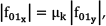
Initially, no sliding is assumed and the state is static friction ( ${\mathrm{x}}_1=0;\mathrm{\hspace{0.17em}}{\stackrel{.}{\mathrm{x}}}_1=0;\mathrm{\hspace{0.17em}}{\stackrel{..}{\mathrm{x}}}_1=0)$ . Thus, solving Eq. (6), the values of f01x (friction force) and f01y (normal force) are obtained. Next, the static friction condition Eq. (7) is evaluated for a specified static friction coefficient, ${\mathrm{\mu }}_{\mathrm{s}}$ :

$\left|{\mathrm{f}}_{{01}_{\mathrm{x}}}\right|\le {\mathrm{\mu }}_{\mathrm{s}}\left|{\mathrm{f}}_{{01}_{\mathrm{y}}}\right|$

(7)

If Eq. (7) is satisfied, the time is incremented by ∆t and Eq. (6) is recalculated using the updated values of ${\mathrm{r}}_{\mathrm{i}\mathrm{j}},\mathrm{\hspace{0.17em}}{\stackrel{..}{\mathrm{x}}}_{\mathrm{i}},\mathrm{\hspace{0.17em}}{\stackrel{..}{\mathrm{y}}}_{\mathrm{i}},\mathrm{\hspace{0.17em}}{\stackrel{..}{\mathrm{\vartheta }}}_{\mathrm{i}}$ . This step closes the ‘static friction’ conditional loop.

If Eq. (7) is false, the supporting foot enters the state of imminent slipping and a different system of equations must be solved. This system must accommodate the following conditions: First, since the acceleration of the supporting foot is no longer zero but unknown, it must appear in the column vector of unknowns. Second, the kinetic frictional relationship between normal and tangential components of the floor-foot force must be considered:

$\left|{\mathrm{f}}_{{01}_{\mathrm{x}}}\right|={\mathrm{\mu }}_{\mathrm{k}}\left|{\mathrm{f}}_{{01}_{\mathrm{y}}}\right|,$

(8)

where ${\mathrm{\mu }}_{\mathrm{k}}$ is the kinetic friction coefficient.

The new matrix of coefficients is then obtained from its predecessor by adding the following:

• –

  A column of mi elements in positions corresponding to the x-components of Newton's equations, described in Eq. (4), with zeroes elsewhere;

• –

  An additional row incorporating Eq. (8).

Therefore, the final matrix form of the ‘inverse dynamic sliding friction equation’ is as follows:

The sign of the friction force exerted by the floor on the supporting foot varies (hence the designation ±μk in Eq. 9) depending on the sliding status in the previous calculation. When the previous state was imminent sliding, the friction force opposes the horizontal component of the other forces acting on the foot, and sign μk = sign ( ${\mathrm{f}}_{12\mathrm{x}\mathrm{\hspace{0.17em}}}+\mathrm{\hspace{0.17em}}{\mathrm{f}}_{\mathrm{1,12}\mathrm{x}}$ ).

Having solved Eq. 9, the program returns the acceleration with which the supporting foot has begun sliding, ${\stackrel{..}{\mathrm{x}}}_1$ . In the current time interval ( $\left(\mathrm{n}-1\right)∆\mathrm{T}$ – $\mathrm{n}∆\mathrm{t}$ ), the supporting foot is assumed to move with the calculated uniform acceleration. The velocity and position of the supporting foot are then updated by Eq. (10):

$\begin{array}{c}{\stackrel{..}{\mathrm{x}}}_1\text{=}\mathrm{c}\mathrm{t}\mathrm{e}.\hspace{0.17em}\mathrm{i}\mathrm{n}\hspace{0.17em}\mathrm{t}\mathrm{h}\mathrm{e}\hspace{0.17em}\mathrm{i}\mathrm{n}\mathrm{t}\mathrm{e}\mathrm{r}\mathrm{v}\mathrm{a}\mathrm{l}\hspace{0.17em}\text{∆}\mathrm{t}\\ {\stackrel{.}{\mathrm{x}}}_1\left[\mathrm{n}∆\mathrm{t}\right]={\stackrel{.}{\mathrm{x}}}_1\left[\left(\mathrm{n}-1\right)∆\mathrm{t}\right]+{\stackrel{..}{\mathrm{x}}}_1∆t\\ {\mathrm{x}}_1\left[\mathrm{n}∆\mathrm{t}\right]={\mathrm{x}}_1\left[\left(\mathrm{n}-1\right)∆\mathrm{t}\right]+{\stackrel{.}{\mathrm{x}}}_1\left[\left(\mathrm{n}-1\right)∆\mathrm{t}\right]·∆t+{\frac{1}{2}\stackrel{..}{\mathrm{x}}}_1{\left(∆\mathrm{t}\right)}^2\end{array}$

(10)

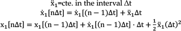
Here, the square brackets indicate functional dependence. After performing the above calculation, the program stores the force and torque data, as well as the kinematic data for all links, increments the time by $∆\mathrm{t}$ and re-solves Eq. 9. Now, since the foot is already sliding, the friction force opposes the foot velocity and sign μk = – sign ${\stackrel{.}{\mathrm{x}}}_1$ .

Whenever the supporting foot is sliding, the floor exerts an opposing friction force. This force can halt the supporting foot in the given time interval, but cannot change the direction of sliding. To accommodate this rule, the program calculates the stopping time, ts, and compares it with the time increment, $∆\mathrm{t}$ , as shown in Eq. (11).

${\mathrm{t}}_{\mathrm{s}}=-\frac{{\stackrel{.}{\mathrm{x}}}_1}{{\stackrel{..}{\mathrm{x}}}_1}$

(11)

If ts is negative or exceeds $∆\mathrm{t}$ , the supporting foot continues sliding at the end of the time interval. On the other hand, if ts is positive and less than $∆\mathrm{t}$ , then friction halts the supporting foot before the end of the time interval. In this case, the program updates positions and velocities using ts instead of ∆t, and returns to the beginning to solve the case of static friction, Eq. (6).

Fig. 4 is a flowchart of the inverse dynamics program. ‘Dynamical unknowns’ (forces between links and torque T8) are stored during the ‘STORING DATA’ task. Kinematic variables for the supporting foot are updated according to Eq. (10), and for the rest of the links by Eqs. (2) to (4 bis).

Figure 4.

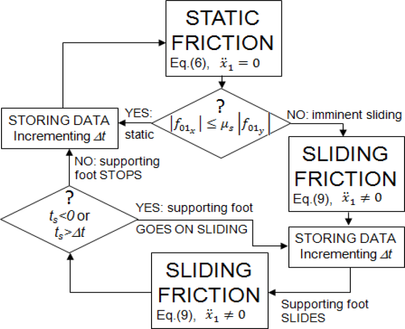
Flowchart of the program for calculating inverse dynamics and sliding supporting foot

4.3. Forward Dynamics and Fixed Supporting Foot

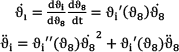
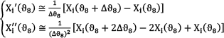
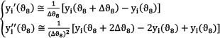
When addressing forward dynamics, the kinematics is unknown. However, the angular position of the motor crank defines the position of the remaining links by Eqs. (1)– (3). These functions were defined in [1]. The corresponding angular velocities and accelerations as well as the centre of mass linear velocities and accelerations are obtained from the first and second time derivatives:

$\begin{array}{c}\stackrel{.}{{\mathrm{\vartheta }}_{\mathrm{i}}}=\frac{\mathrm{d}{\mathrm{\vartheta }}_{\mathrm{i}}}{\mathrm{d}{\mathrm{\vartheta }}_8}\frac{\mathrm{d}{\mathrm{\vartheta }}_8}{\mathrm{d}\mathrm{t}}={\mathrm{\vartheta }}_{\mathrm{i}}^{\mathrm{\prime }}\left({\mathrm{\vartheta }}_8\right)\stackrel{.}{{\mathrm{\vartheta }}_8}\\ {\stackrel{..}{\mathrm{\vartheta }}}_{\mathrm{i}}={\mathrm{\vartheta }}_{\mathrm{i}}^{\mathrm{\prime }\mathrm{\prime }}\left({\mathrm{\vartheta }}_8\right){\stackrel{.}{{\mathrm{\vartheta }}_8}}^2+{\mathrm{\vartheta }}_{\mathrm{i}}^{\mathrm{\prime }}\left({\mathrm{\vartheta }}_8\right){\stackrel{..}{\mathrm{\vartheta }}}_8\end{array}$

(12)

$\begin{array}{c}\stackrel{.}{{\mathrm{X}}_{\mathrm{i}}}={\mathrm{X}}_{\mathrm{i}}^{\mathrm{\prime }}\left({\mathrm{\vartheta }}_8\right)\stackrel{.}{{\mathrm{\vartheta }}_8}\\ {\stackrel{..}{\mathrm{X}}}_{\mathrm{i}}={\mathrm{X}}_{\mathrm{i}}^{\mathrm{\prime }\mathrm{\prime }}\left({\mathrm{\vartheta }}_8\right){\stackrel{.}{{\mathrm{\vartheta }}_8}}^2+{\mathrm{X}}_{\mathrm{i}}^{\mathrm{\prime }}\left({\mathrm{\vartheta }}_8\right){\stackrel{..}{\mathrm{\vartheta }}}_8\end{array}$

(13)

$\begin{array}{c}\stackrel{.}{{\mathrm{y}}_{\mathrm{i}}}={\mathrm{y}}_{\mathrm{i}}^{\mathrm{\prime }}\left({\mathrm{\vartheta }}_8\right)\stackrel{.}{{\mathrm{\vartheta }}_8}\\ {\stackrel{..}{\mathrm{y}}}_{\mathrm{i}}={\mathrm{y}}_{\mathrm{i}}^{\mathrm{\prime }\mathrm{\prime }}\left({\mathrm{\vartheta }}_8\right){\stackrel{.}{{\mathrm{\vartheta }}_8}}^2+{\mathrm{y}}_{\mathrm{i}}^{\mathrm{\prime }}\left({\mathrm{\vartheta }}_8\right){\stackrel{..}{\mathrm{\vartheta }}}_8\end{array}$

(14)

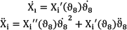
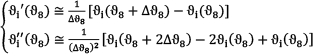
When the kinematics is unknown, Eq. (5) becomes a system of second order differential equations. To solve it numerically, in addition to time, the motor crank angle ϑ8 is discretized. In this way, the derivatives of the known functions, ϑi = ϑi (ϑ8), Xi = Xi (ϑ8) and yi = yi (ϑ8), are computed with respect to ϑ8:

$\left\{\begin{array}{l}{\mathrm{\vartheta }}_{\mathrm{i}}^{\mathrm{\prime }}\left({\mathrm{\vartheta }}_8\right)\cong \frac{1}{∆{\mathrm{\vartheta }}_8}\left[{\mathrm{\vartheta }}_{\mathrm{i}}\left({\mathrm{\vartheta }}_8+∆{\mathrm{\vartheta }}_8\right)-{\mathrm{\vartheta }}_{\mathrm{i}}\left({\mathrm{\vartheta }}_8\right)\right]\\ {\mathrm{\vartheta }}_{\mathrm{i}}^{\mathrm{\prime }\mathrm{\prime }}\left({\mathrm{\vartheta }}_8\right)\cong \frac{1}{{\left(∆{\mathrm{\vartheta }}_8\right)}^2}\left[{\mathrm{\vartheta }}_{\mathrm{i}}\left({\mathrm{\vartheta }}_8+2∆{\mathrm{\vartheta }}_8\right)-2{\mathrm{\vartheta }}_{\mathrm{i}}\left({\mathrm{\vartheta }}_8\right)+{\mathrm{\vartheta }}_{\mathrm{i}}\left({\mathrm{\vartheta }}_8\right)\right]\end{array}\right.$

(12 bis)

$\left\{\begin{array}{l}{\mathrm{X}}_{\mathrm{i}}^{\mathrm{\prime }}\left({\mathrm{\vartheta }}_8\right)\cong \frac{1}{∆{\mathrm{\vartheta }}_8}\left[{\mathrm{X}}_{\mathrm{i}}\left({\mathrm{\vartheta }}_8+∆{\mathrm{\vartheta }}_8\right)-{\mathrm{X}}_{\mathrm{i}}\left({\mathrm{\vartheta }}_8\right)\right]\\ {\mathrm{X}}_{\mathrm{i}}^{\mathrm{\prime }\mathrm{\prime }}\left({\mathrm{\vartheta }}_8\right)\cong \frac{1}{{\left(∆{\mathrm{\vartheta }}_8\right)}^2}\left[{\mathrm{X}}_{\mathrm{i}}\left({\mathrm{\vartheta }}_8+2∆{\mathrm{\vartheta }}_8\right)-2{\mathrm{X}}_{\mathrm{i}}\left({\mathrm{\vartheta }}_8\right)+{\mathrm{X}}_{\mathrm{i}}\left({\mathrm{\vartheta }}_8\right)\right]\end{array}\right.$

(13 bis)

$\left\{\begin{array}{l}{\mathrm{y}}_{\mathrm{i}}^{\mathrm{\prime }}\left({\mathrm{\vartheta }}_8\right)\cong \frac{1}{∆{\mathrm{\vartheta }}_8}\left[{\mathrm{y}}_{\mathrm{i}}\left({\mathrm{\vartheta }}_8+∆{\mathrm{\vartheta }}_8\right)-{\mathrm{y}}_{\mathrm{i}}\left({\mathrm{\vartheta }}_8\right)\right]\\ {\mathrm{y}}_{\mathrm{i}}^{\mathrm{\prime }\mathrm{\prime }}\left({\mathrm{\vartheta }}_8\right)\cong \frac{1}{{\left(∆{\mathrm{\vartheta }}_8\right)}^2}\left[{\mathrm{y}}_{\mathrm{i}}\left({\mathrm{\vartheta }}_8+2∆{\mathrm{\vartheta }}_8\right)-2{\mathrm{y}}_{\mathrm{i}}\left({\mathrm{\vartheta }}_8\right)+{\mathrm{y}}_{\mathrm{i}}\left({\mathrm{\vartheta }}_8\right)\right]\end{array}\right.$

(14 bis)

In fact, to implement the forward dynamic problem, Eqs. (12), (13), (14), (12 bis), (13 bis) and (14 bis) are inserted into Eq. (5). Thus, we obtain a system of equations in which the first and second time derivatives of ϑ8 are unknown, while the torque is now a known function of time, T8 = T8 (t). The resulting system of equations is as follows:

$\{\begin{array}{l}{\displaystyle \sum _{j<i}{f}_{j{i}_x}-}{\displaystyle \sum _{k>i}{f}_{i{k}_x}}-m_i{X}_{\mathrm{i}}^{\mathrm{\prime }}\left({\vartheta }_8\right){\stackrel{..}{\vartheta }}_8=m_i{X}_{\mathrm{i}}^{\mathrm{\prime }\mathrm{\prime }}\left({\vartheta }_8\right){\stackrel{.}{\vartheta }}_8{}^2\\ {\displaystyle \sum _{j<i}{f}_{j{i}_y}-}{\displaystyle \sum _{k>i}{f}_{i{k}_y}}-m_i{y}_{\mathrm{i}}^{\mathrm{\prime }}\left({\vartheta }_8\right){\stackrel{..}{\vartheta }}_8=m_{i}g+m_i{y}_{\mathrm{i}}^{\mathrm{\prime }\mathrm{\prime }}\left({\vartheta }_8\right){\stackrel{.}{\vartheta }}_8{}^2\\ {\displaystyle \sum _{j<i}{T}_{ji}-}{\displaystyle \sum _{k>i}{T}_{ik}}+{\displaystyle \sum _{j<i}\left(r_{i{j}_x}{f}_{j{i}_y}-r_{i{j}_y}{f}_{j{i}_x}\right)-}\\ -{\displaystyle \sum _{k>i}\left(r_{i{k}_x}{f}_{i{k}_y}-r_{i{k}_y}{f}_{i{k}_x}\right)-I_i{\mathrm{\vartheta }}_{\mathrm{i}}^{\mathrm{\prime }}\left({\vartheta }_8\right){\stackrel{..}{\vartheta }}_8=I_i{\mathrm{\vartheta }}_{\mathrm{i}}^{\mathrm{\prime }\mathrm{\prime }}\left({\vartheta }_8\right){\stackrel{.}{\vartheta }}_8{}^2}\end{array}$

(15)

The numerical approach used to solve the system of differential equations Eq. (15) involves a time discretization. At each time step, a linear inhomogeneous system is solved, where the forces between links (fjix, fjiy), and the angular acceleration of the motor crank, ${\stackrel{..}{\mathrm{\vartheta }}}_8$ , are unknown, while the angular speed of the motor crank, ${\stackrel{.}{\mathrm{\vartheta }}}_8$ , is known. Meanwhile, ${\stackrel{.}{\mathrm{\vartheta }}}_8$ is assigned an initial value ${\stackrel{.}{\mathrm{\vartheta }}}_8\left(\mathrm{t}=0\right)$ , which is updated after solving Eq. (15) in the previous time step. Regarding the determined angular acceleration as constant during ∆t, the updated angular velocity is as follows:

${\stackrel{.}{\mathrm{\vartheta }}}_8\left[\mathrm{n}∆\mathrm{t}\right]={\stackrel{.}{\mathrm{\vartheta }}}_8\left[\left(\mathrm{n}-1\right)∆\mathrm{t}\right]+{\stackrel{..}{\mathrm{\vartheta }}}_8∆\mathrm{t}$

(16)

Thus, the coefficient matrix is obtained from that of Eq. 9 by eliminating the column corresponding to the torque coefficients T8 (previously unknown), and adding a column representing the coefficients of the motor crank angular acceleration, ${\stackrel{..}{\mathrm{\vartheta }}}_8$ (now unknown). The torque T8 must now be included in the column of constants. Thus, the matrix form of Eq. (15), the ‘forward dynamics equation’ is obtained as follows:

$\begin{array}{l}A=\left[\begin{array}{ccccc}{a}_{11}& a_{12}& \cdots & a_{\mathrm{1,71}}& 0\\ a_{21}& a_{22}& \cdots & a_{\mathrm{2,71}}& 0\\ a_{31}& a_{32}& \cdots & a_{\mathrm{3,71}}& -m_2{x}_2{\hspace{0.17em}}^{\mathrm{\prime }}({\vartheta }_8)\\ a_{41}& a_{42}& \cdots & a_{\mathrm{4,71}}& -m_2{y}_2{\hspace{0.17em}}^{\mathrm{\prime }}({\vartheta }_8)\\ a_{51}& a_{52}& \cdots & a_{\mathrm{5,71}}& -I_2{\vartheta }_2{\hspace{0.17em}}^{\mathrm{\prime }}({\vartheta }_8)\\ ⋮& ⋮& \ddots & ⋮& ⋮\\ a_{\mathrm{71,1}}& a_{\mathrm{71,2}}& \cdots & a_{\mathrm{71,71}}& -I_{{12}^{\mathrm{\prime }}}{\vartheta }_{{12}^{\mathrm{\prime }}}({\vartheta }_8)\end{array}\right]\\ \mathrm{U}=\left[\begin{array}{c}{f}_{01x}\\ f_{01y}\\ f_{12x}\\ f_{12y}\\ ⋮\\ .\\ f_{{10}^{\mathrm{\prime }},{12}^{\mathrm{\prime }}y}\\ {\stackrel{..}{\vartheta }}_8\end{array}\right];C=\left[\begin{array}{c}0\\ m_{1}g\\ m_2{X}_2{\hspace{0.17em}}^{\mathrm{\prime }\mathrm{\prime }}\left({\vartheta }_8\right){\stackrel{.}{\vartheta }}_8{}^2\\ m_{2}g+m_2{y}_2{\hspace{0.17em}}^{\mathrm{\prime }\mathrm{\prime }}\left({\vartheta }_8\right){\stackrel{.}{\vartheta }}_8{}^2\\ I_2{\vartheta }_2{\hspace{0.17em}}^{\mathrm{\prime }\mathrm{\prime }}\left({\vartheta }_8\right){\stackrel{.}{\vartheta }}_8{}^2\\ ⋮\\ T_8\\ \\ \end{array}\right]\\ \left[A(\text{coeff.\hspace{0.17em}})\right]·\left[U(\text{forces},{\stackrel{..}{\vartheta }}_8)\right]=\left[C(\text{cts})\right]\Rightarrow \left[U\right]={\left[A\right]}^{-1}·\left[C\right]\end{array}$

(17)

4.4. Forward Dynamics and Sliding Supporting Foot

Here, sliding of the supporting foot is treated as in 3.2, whereas the forward dynamics is formulated as in 3.3. The flowchart presented in Fig. 4 is essentially maintained, but the systems of equations to be solved at each stage are different:

• –

  In the state of ‘STATIC FRICTION’ the system to be solved is the forward dynamics system of Eq. (17), referred to as the ‘static system (ST)’.

• –

  In the state of ‘SLIDING FRICTION’, an equation describing the sliding supporting foot, Eq. (8), and a new unknown, ${\stackrel{..}{\mathrm{x}}}_1$ , are added to Eqs. (17). Moreover, the penultimate and final elements of the unknowns column become the motor crank angular acceleration and the supporting foot sliding acceleration, respectively. Meanwhile, the torque T8 appears in the constants column. The first and second derivatives of Xi, yi and ϑi with respect to ϑ8 are calculated beforehand using Eqs. (12bis)– (14bis), with a sufficiently fine discretization of ϑ8. The resulting system of equations (17 bis) is referred to as the ‘sliding system (SL)’.

• –

  In ‘STORING DATA’ mode, the kinematics of the supporting foot is updated by Eq. (10). The motor crank position and velocity is updated according to Eq. (16), followed by the update of the remaining links using Eqs. (12)– (14 bis).

4.5. Double Support Phase

To conclude the dynamics of PASIBOT, in this section, we outline the algorithm that solves PASIBOT's movement when both feet contact the floor. This phase is non-negligible, since it consumes a quarter of a complete time step for a constant value of the motor crank velocity. Furthermore, kinematic analysis indicates that during this phase, a slight longitudinal relative displacement occurs between both feet, so that at any given moment one of the following actions is possible:

• a)

  The back foot (for example, link 1) is static, while the front foot (link 1') slides;

• b)

  Both feet slide on the floor;

• c)

  The back foot slides and the front one does not.

Which situation occurs depends upon the normal force exerted by the ground on each foot. In fact, throughout the double support phase, the three actions occur in the order shown, since the normal force is transferred from the back foot (initially the only foot in contact with the floor) to the front foot (which supports the entire normal force when the back foot leaves the floor). The instances at which a change of action occurs also depend on the friction coefficient; large μk will invoke situations a) and c) at the expense of b), and vice versa.

To solve the forward dynamics of the double support phase, two additional unknowns (and their corresponding equations) are required. The unknowns are the contact (friction and normal) forces exerted by the floor on the front foot, f01'x and f01'y, which occupy two extra columns in the coefficient matrix of Eq. (17). The new equations occupy two additional rows in the same matrix. One equation describes the vertical force equilibrium (note that, as stated in [1], the biped centre of mass has no vertical acceleration):

${\mathrm{f}}_{{01}_{\mathrm{y}}}+{\mathrm{f}}_{{{01}^{\mathrm{\prime }}}_{\mathrm{y}}}=\mathrm{M}\mathrm{g}$

(18)

The second equation describes kinetic friction, which depends on the invoked action (a, b or c):

• a)

  If the back foot is static while the front foot slides, the “static system (ST)” must be solved, together with the kinetic friction equation for the front foot:

  $\left|{\mathrm{f}}_{{{01}^{\mathrm{\prime }}}_{\mathrm{x}}}\right|={\mathrm{\mu }}_{\mathrm{k}}\left|{\mathrm{f}}_{{{01}^{\mathrm{\prime }}}_{\mathrm{y}}}\right|$

  (19)

• b)

  If both feet slide, the ‘sliding system (SL)’ must be solved, together with the kinetic friction equation for the front foot (Eq. (19)).

• c)

  If the back foot slides while the front foot is static, case a) must be solved after permuting the foot labels (1 ↔ 1').

The flowchart outlining the double support phase forward dynamics is displayed as Fig. 5.

Figure 5.

Flowchart of the program for calculating double support forward dynamics

5. Results and discussion

As extensions of the code developed in [1], the kinematic and dynamic algorithms presented in the previous sections were implemented in MATLAB. In [1], steady inverse dynamics and fixed supporting foot were assumed. Here, we present results from the developed forward dynamics model. We also consider sliding at different friction coefficients and motor crank velocities.

Forward dynamics is particularly valuable in transient calculations; for example, computing the minimum constant torque applied to the motor crank for PASIBOT to start walking from rest. In Fig. 6, the motor crank angle is plotted against time for a range of motor torques.

Figure 6.

Evolution of the motor crank angle for different motor torques, when the biped starts walking from rest, according to the program described in this article

As shown in Fig. 6, the torque above which the biped can start walking is 0.84 Nm. Note that the initial value of ${\mathrm{\vartheta }}_8$ is π/2, corresponding to the configuration in which both feet are on the floor. In this example, the density of all links is the same as that of aluminium, from which the prototype is built.

These results were compared with those obtained with the software Working Model 2D. Comparing Figs. 6 and 7, we can say that the results are similar enough to each other to validate the program described in this article.

Figure 7.

Evolution of the motor crank angle for different motor torques, when the biped starts walking from rest, according to Working Model 2D simulations

The program allows the density of any link to be easily changed. In this way, the extent to which density affects the minimum required torque can be determined. In Fig. 8, the motor crank angle is plotted as a function of time for a constant motor torque, T₈ = 1 Nm and varying total weight (obtained by varying the density of all links).

Figure 8.

Evolution of the motor crank angle when the biped starts walking from rest, for a constant motor torque, T₈ = 1 Nm, and for different total weights

Fig. 9 plots the horizontal supporting foot position as a function of time for a constant motor crank angular velocity, ${\stackrel{.}{\mathrm{\vartheta }}}_8=3\mathrm{\hspace{0.17em}}\mathrm{r}\mathrm{a}\mathrm{d}/\mathrm{s}$ , and varying friction coefficient (here μ_s = μ_k ≡ μ). From this plot, we can deduce the time course of the supporting foot sliding.

Figure 9.

x-coordinate of the supporting foot versus time (in units of one period, T) for constant ${\stackrel{.}{\mathrm{\vartheta }}}_8=3\mathrm{\hspace{0.17em}}\mathrm{r}\mathrm{a}\mathrm{d}/\mathrm{s}$ , varying friction coefficient μ and ∆t=T/15

From Fig. 9, we first observe that the minimum friction coefficient that prevents the supporting foot from sliding is 0.08. Second, sliding occurs during preferred phases. Thus, if the supporting foot slides once during a step (Fig. 8; μ = 0.06), sliding starts at mid-step (t=0.5T) to when the swinging leg has reached its highest point, t = 0.6T. If two slippages occur (Fig. 9; μ = 0.04), one of them is again invoked at mid-step, while the other occurs at the first quarter-step (from t = 0.15T to t = 0.25T). For μ = 0.03, slippage occurs repeatedly at various phases.

Fig. 10 shows the sliding characteristics for constant friction coefficient μ = 0.1 but different motor crank angular velocities.

Figure 10.

x-coordinate of the supporting foot versus time (in units of one period, T) for μ = 0.1, varying ${\stackrel{.}{\mathrm{\vartheta }}}_8$ and ∆t=T/15

As for Fig. 9, step phases where the supporting foot is likely to slide are evident in Fig. 10. These results suggest that slippage may be drastically reduced, or perhaps eliminated, without compromising step speed, by reducing the angular velocity at the ‘easy slippage phases’ and increasing it at other times, i.e., by defining an appropriate time-dependent function of the motor angular velocity time function, ${\stackrel{.}{\mathrm{\vartheta }}}_8={\stackrel{.}{\mathrm{\vartheta }}}_8\left(\mathrm{t}\right)$ .

The program allows for the setting of different values for static and kinetic friction coefficients (in practice, static friction coefficient is bigger than kinetic friction coefficient, μ_s > μ_k). Fig. 11 shows the supporting foot sliding for the same static friction coefficient, μ_s = 0.2, and three different values for the kinetic friction coefficient, μ_k = 0.2, 0.1 and 0.05.

Figure 11.

x-coordinate of the supporting foot versus time for constant ${\stackrel{.}{\mathrm{\vartheta }}}_8=5\mathrm{\hspace{0.17em}}\mathrm{r}\mathrm{a}\mathrm{d}/\mathrm{s}$ , and ∆t=T/15, for the same static friction coefficient, μ_s = 0.2, and for three different kinetic friction coefficients

As can be seen, slippage occurs at the same point for all three cases, whereas, as expected, the lower the kinetic friction coefficient, the greater the sliding distance.

6. Conclusions

We have presented the kinematics and dynamics (both forward and inverse) of the biped robot PASIBOT, accounting for sliding between the supporting foot and the floor during single and double support phases. From these models, we have generated MATLAB algorithms to complete and improve the work initiated in the previous study. The program was applied to movements of PASIBOT in transients and for time-varying torques. In addition, the program calculates the position of the ZMP and identifies potential toppling situations.

The program remains parametric, so that dimensions, masses and densities of links, motor angular velocity or motor torque (in the inverse and forward dynamics versions, respectively), friction coefficients and other parameters can be entered by the user as constants or even as time functions. Thus, using the improved program, we could determine the torque required at the motor/brake to start/stop walking, and hence select suitable actuator and transmission systems.

The developed code has been used to investigate PASIBOT behaviour prior to construction, reducing complexity in the design process, and will be used in control tasks of real prototype walking. Furthermore, the presented program will enable the design of time functions for the angular velocity of the crank motor by which slipping can be reduced in a systematic rather than an ad hoc way, or perhaps eliminated.

By incorporating these extensions into the MATLAB code presented in [1], we have significantly improved our algorithm.